Formal Comparisons of Legislative Institutions: Ideal
Points from Brazilian Legislatures
*Robert Myles McDonnell
Universidade de São Paulo, Brazil
As the popularity of formal analyses of legislative activity in
Latin America grows, so does the importance of understanding the
limits of the estimates produced by such analyses and the
methodological adaptations necessary when using these measures
to make formal comparisons. This research note details the
considerations involved and demonstrates their significance with
an empirical example using the Brazilian Chamber of Deputies and
the Federal Senate. This empirical analysis leads to conclusions that
are the opposite of those in the literature, suggesting that such formal comparisons across institutions need to be made with care.
Keywords: Ideal points; legislative voting; Bayesian
item-response; Federal Senate; Chamber of Deputies.
* http://dx.doi.org/10.1590/1981-3821201700010007
hen making formal comparisons of legislative arenas, there are
methodological considerations that researchers must keep in
mind. In this research note, I outline these concerns and demonstrate with an
example how findings can change once these considerations are taken into
account. By formal comparison, I mean quantitative estimates of legislative voting
behaviour, such as ideal points. As the "primary use of roll call data […] is the
estimation of ideal points" (CLINTON, JACKMAN, and RIVERS, 2004, p. 01), I focus
on these particular estimates throughout this research note. The empirical
example I use is a comparison of ideal point estimates from the Brazilian Chamber
of Deputies and Federal Senate. The present study is part of a wider literature
seeking to correct for measurement errors in latent variable models. Presently, the
context is comparison, but scholars have endeavored to make improvements to
measures of democracy (JACKMAN and TREIER, 2008), how changing standards
affect measurements (FARISS, 2014), and to improve how we measure
transparency (HOLLYER et al., 2014).
Calling attention to the difficulties in making formal comparisons across
legislative arenas or similar institutions is not new. Bailey (2007) and Treier
(2011) both highlight the misleading inferences that may result from comparisons
of this sort when scholars do not include the methodological adaptations
necessary. In fact, these adaptations are conceptually very simple. If we consider
the basic Bayesian Item-Response Theory (IRT) model, employed in this context by
Clinton et al. (2004) and others, we can see clearly the basic requirements for
making valid comparisons of different institutions. This model may be written as:
�( = ) = Φ −
where is a matrix of recorded nominal votes, with i indexing legislators and j
votes, in which = indicates that legislator i voted 'yes' on proposal j, and =
otherwise. Φ is the cumulative normal distribution function, leading to a probit
model. is the 'discrimination' parameter of the model and the 'difficulty'
parameter; is the ideal point of legislator i, which may be understood as her
preferred location in the policy space, a space of usually of one or two dimensions
(JACKMAN, 2001). In regression terms, is the intercept and the slope; this is a
latent regression model, as we only observe .
This model originally comes from the literature on educational tests, the
context of which makes it very clear what is necessary in order to produce
comparable ideal points. The model is designed to gauge the worth of an
educational test, for example, on mathematical ability. The questions may range in
terms of difficulty, and if individuals of varying aptitude in the latent trait
(mathematical ability) answer the same questions in the same manner, these
questions are unable to discriminate between the test-takers. That is, test-takers
who have different levels of ability will have the same probability of answering the
question correctly for questions with low discrimination parameter values.
Questions that can separate individuals of differing capacity do discriminate
between test-takers, and result in the model predicting that individuals of greater
ability have a higher probability of answering correctly.
Although ideal points are not usually the main items of interest in this
literature, with this model we can recover estimates of where the test-takers are
positioned on the latent trait scale. For tests that discriminate well, we would
expect to find those of limited mathematical skill at one end of the scale, while
those with higher levels should be found at the other.
In the present context, the scale is constructed from the voting behavior of
the legislators as compared to one another; two legislators who never vote the
same way will be on the two extremes of the scale, for example, whereas those who
vote similarly will be placed along the same region. The positions of the legislators
on the scale are their ideal points. High absolute values of the discrimination
parameter (above two or below minus two) indicate that the proposal separated
the legislators; in other words, all the legislators do not vote in the same way for
proposals with these high values. Conversely, values of this parameter that are
close to zero indicate that all or most of the legislators voted the same way on such
proposals.
It is obvious from this short description that test-takers must answer the
same questions in order for their positions on the scale to be comparable. In the
political context, we may not have the same control over what 'questions' (votes)
legislators respond to, but this requirement remains the same. Hence, to compare
two different institutions, both sets of legislators must respond to the same bills.
may not be justifiable: legislators in different houses may vote on very different
versions of the same bill, for example, and bills may be amended many times
before arriving in one house from the other. With regard to time, analyses of ideal
points usually take a single legislature as a unit of analysis. Extending the period of
time may necessitate the need for a dynamic model, such as that of Martin and
Quinn (2002).
To expand upon this theme, I use the example of a comparison of ideal
points between the Chamber of Deputies and the Federal Senate in Brazil, with the
dataset from CEBRAP Legislative Dataset. These two houses have been formally
compared by Freitas, Izumi, and Medeiros (2012), Bernabel (2015) and Desposato
(2006). Desposato (2006) utilizes the fact that deputies and senators vote
sequentially in the National Congress to place both sets of legislators in a common
space. This is the most valid method for doing so, and cleverly exploits a native
feature of the Brazilian political system. However, as Bailey (2007) notes, votes
must be coded as being the same item, as if they were the exact same question in an
educational-testing context (BAILEY, 2007, p. 440); there is no evidence available
that Desposato (2006) undertook this necessary step. Freitas et al. (2012) estimate
ideal point means for both houses separately and then compare the means, which
is not a valid method of formal comparison; Bernabel (2015) estimates ideal points
for both houses separately, which is also invalid as a method of comparison, and
although the study is offered as a descriptive piece (BERNABEL, 2015, p. 106), this
comparison is potentially quite misleading. For example, Desposato (2006) finds
less party cohesion in the Senate when compared to the Chamber, whereas
Bernabel (2015) finds the opposite – how are we to know which finding is correct?
To productively compare these houses, we must place both on a common
scale, as noted by Bernabel (2015). In order to do so, we must know which
proposals were voted on in both houses, and on which versions of the proposals
the houses voted, and which are common to both houses. Exactly how to do so will
differ on the specific context. In the current example, we can exploit the common
votes in the National Congress and use these votes as a means to 'bridge' between
the two houses. These votes are coded as being the same item in the database and
votes. The analysis may then proceed using all the remaining votes from both
houses in one common dataset.
This method is the same as that proposed by Desposato (2006), but leads
to opposite findings. As mentioned previously, there is no evidence that Desposato
(2006) treated the common votes in the National Congress as the exact same item,
and I can only surmise that the difference in the findings presented here is down to
this important detail.
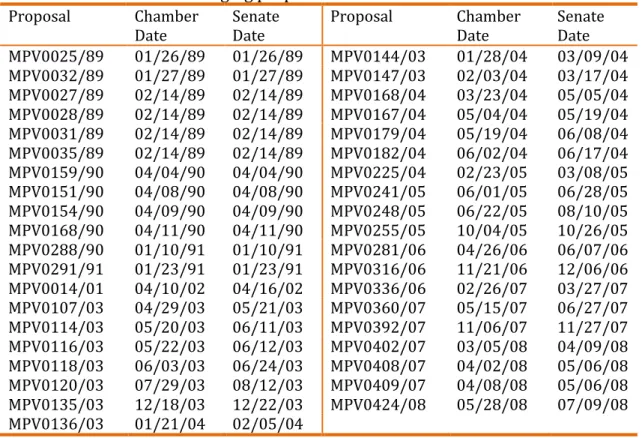
The specific set of votes that were used to bridge the houses is that of the
Medidas Provisórias (MPVs, Provisional Decrees) issued by the Executive and
voted on in the National Congress. Many of these votes happened sequentially,
although in a few cases the vote in the Senate happened at a later date (see Table
1). However, given that the voting is indeed sequential in the National Congress
(DESPOSATO, 2006), it is therefore not perfectly simultaneous, and this difference
in time between the houses should not make any obvious difference. The Senators
are aware of the result of the Deputies' votes in either case, and while it may be
possible that the external political context shifted so rapidly as to change the
probability of a 'yes' vote in the second house, this is unlikely for the small number
of MPVs involved in the years analyzed (1989-2010). All other non-unanimous
votes in both houses were then used in the normal manner, from one large
conjoined dataset, once the bridging votes were coded as such.
There are of course other ways to bridge legislatures. One method is to use
the legislators themselves, as in Shor et al. (2010). In the Brazilian case, voting
behavior could be analyzed over several levels of government – from
municipalities to federal legislatures, and as such is an interesting avenue for
future research, but not the focus of the present research note. Another method is
to use the content of the votes themselves and thus code votes on the same
proposal that occur in different time periods as a means to bridge over time, as in
Bailey et al. (2015); future studies on the dynamics of voting in both the Chamber
and Senate could utilize this method.
Once we place the deputies and senators in a common space, we can
meaningfully analyze hypotheses of differences between the institutions,
operationalized by examining ideal point estimates from this common scale. Due to
ideal points are considered below for both houses. Claims in the literature lead to
several hypotheses, the first being H1: there is no significant difference in voting
behavior across the two houses, as argued by Desposato (2006). This can be
operationalized by examining the difference in means of the ideal points in both
houses and the magnitude of the difference through a Bayesian version of the
't-test' for two groups (KRUSCHKE, 2013).
Table 01. Votes used as bridging proposals
Proposal Chamber
Date
Senate Date
Proposal Chamber
Date
Senate Date
MPV0025/89 01/26/89 01/26/89 MPV0144/03 01/28/04 03/09/04
MPV0032/89 01/27/89 01/27/89 MPV0147/03 02/03/04 03/17/04
MPV0027/89 02/14/89 02/14/89 MPV0168/04 03/23/04 05/05/04
MPV0028/89 02/14/89 02/14/89 MPV0167/04 05/04/04 05/19/04
MPV0031/89 02/14/89 02/14/89 MPV0179/04 05/19/04 06/08/04
MPV0035/89 02/14/89 02/14/89 MPV0182/04 06/02/04 06/17/04
MPV0159/90 04/04/90 04/04/90 MPV0225/04 02/23/05 03/08/05
MPV0151/90 04/08/90 04/08/90 MPV0241/05 06/01/05 06/28/05
MPV0154/90 04/09/90 04/09/90 MPV0248/05 06/22/05 08/10/05
MPV0168/90 04/11/90 04/11/90 MPV0255/05 10/04/05 10/26/05
MPV0288/90 01/10/91 01/10/91 MPV0281/06 04/26/06 06/07/06
MPV0291/91 01/23/91 01/23/91 MPV0316/06 11/21/06 12/06/06
MPV0014/01 04/10/02 04/16/02 MPV0336/06 02/26/07 03/27/07
MPV0107/03 04/29/03 05/21/03 MPV0360/07 05/15/07 06/27/07
MPV0114/03 05/20/03 06/11/03 MPV0392/07 11/06/07 11/27/07
MPV0116/03 05/22/03 06/12/03 MPV0402/07 03/05/08 04/09/08
MPV0118/03 06/03/03 06/24/03 MPV0408/07 04/02/08 05/06/08
MPV0120/03 07/29/03 08/12/03 MPV0409/07 04/08/08 05/06/08
MPV0135/03 12/18/03 12/22/03 MPV0424/08 05/28/08 07/09/08
MPV0136/03 01/21/04 02/05/04
Source: CEBRAP Legislative Dataset
Some have posited differences in parties across the two legislatures, in
particular that the PMDB, the 'Partido do Movimento Democrático Brasileiro',
has differing factions depending on the house (ZUCCO JR. and LAUDERDALE,
2011). Our second hypothesis is therefore H2: there is a significant difference in
party voting behavior across houses, in particular the PMDB, which is
operationalized in the same way as H1.
Desposato (2006) and Bernabel (2015) also disagreed on party
cohesion within these legislatures, with the former finding more cohesion in the
Chamber are more cohesive than those of the Senate. In order to examine this
hypothesis, I will employ the same method as before, but with the standard
deviations of party ideal points in the houses rather than party mean ideal
points.
It may also be the case that the Senate votes differently owing to its
purpose (NEIVA, 2013), its specific powers (NEIVA, 2008), the senior and
perhaps conservative profile of the senators themselves (many are former
presidential candidates, governors, party leaders and ex-ministers), or the high
level of unelected suplentes (stand-ins) in the Senate (NEIVA and IZUMI, 2012);
the hypotheses above will allow to establish if there is a difference in voting
behavior between the Senate and the Chamber and its magnitude. These
questions of why there is a difference are an important area for further
research.
In order to test these hypotheses, I utilize methods detailed in Kruschke
(2013), implemented in R with the BEST package (KRUSCHKE and MEREDITH,
2015). In the following discussion, I use the terms 'left' and 'right' as commonly
understood, although the policy space could of course be another scale, such as
government–opposition (IZUMI, 2016).
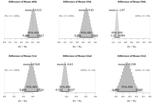
Figure 01 shows the difference in means of ideal points for the two
houses across all six legislatures studied. In each case, the Chamber is 'mean 01'
μ1). The histograms show the posterior probability distribution of the
difference of the mean ideal point of the Chamber minus that of the Senate, with
the 95% Highest Density Interval (HDI) displayed at the base of the histogram.
Were the differences zero in any legislature, we would see that some part of any
one of the histograms touches zero. As can be clearly seen, not only is this not
the case, but all the distributions are quite some distance from zero. Hence
Hypothesis 01 finds no support – voting behavior in the two houses is quite
clearly different, with only Lula's second term in the 53rd legislature coming
anywhere close to zero.
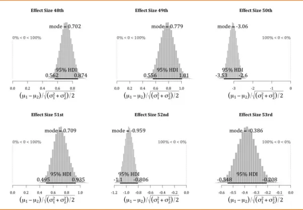
To assess the magnitude of this difference, we can examine the 'effect
size' of the difference in these mean ideal points, which is the difference in the
groups1. Figure 02 shows effect sizes for the six terms considered. Legislatures
48, 49 and 51 – the presidencies of Sarney, Collor, Franco and Cardoso – have
effect sizes of close to 0.7, meaning that there is roughly a 76% probability that
a deputy from these periods was to the right of a senator from the same period2.
Legislature 52, Lula's first term as president, displays an effect size of 0.955,
meaning a probability of 82% that a deputy in this term was more to the right
than a senator. The smallest effect size is to be found in Lula's second term (a
roughly 62% probability), whereas the largest, an enormous -03.06, is found in
Cardoso's first term, in which it is virtually guaranteed (99.9%) that a senator
was more right-wing than a deputy of the same period. These effect sizes
demonstrate that the findings of Desposato (2006), of no clear and consistent
difference between the houses, cannot be supported.
Figure 01. Bayesian t-test of a difference in the means of the ideal points of the Chamber (μ1 and the Senate μ2) for legislatures 48 to 53
Source: CEBRAP Legislative Dataset
Note: The null hypothesis of no difference in means is marked on each plot at the point of zero.
_______________________________________________________________________
1 For each combination of means and standard deviations, the effect size is computed as
� − � /√ � + � / . See Kruschke (2013, p. 08).
Figure 02. Effect sizes for the difference in means between the Chamber and Senate, 48th– 53rd legislatures
Source: CEBRAP Legislative Dataset
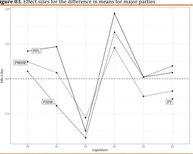
Hypothesis 03 posits a difference in party behavior across the two
institutions, with the literature paying particular reference to upper and
lower house factions of the PMDB. Figure 03 plots the effect sizes of the
differences in parties between the two institutions for the legislatures
considered (the PT is plotted only in the 52nd legislature due to the low
number of senators the party had before this period). As can be readily
observed from the graph, the effect size for the difference in the PMDB
across the two houses is the most moderate of the three large parties, with
this pattern changing only in the 52nd legislature. Among the four parties
graphed, the PFL is the one that seems most split between the houses, at
least until the 52nd legislature. Hence hypothesis 02 receives support for all
Figure 03. Effect sizes for the difference in means for major parties
Source: CEBRAP Legislative Dataset
Note: The PT are shown for the 53rd legislature only due to the low number of senators the
party had before this period.
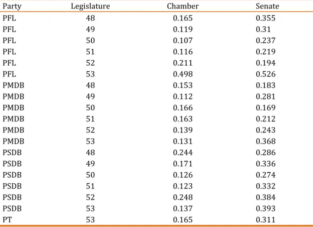
The 'extremity' argument of Bernabel (2015), that senators within each
party vote more for the party than deputies of the same party, is the inverse of
Desposato’s (2006) claim that the parties in the Senate are less cohesive. One way to examine these arguments is to analyze the standard deviations of the t-test for a
difference between the party means of both houses. Greater standard deviations
translate to less cohesion, as the ideal points of the individuals in the party are
more spread out in this case. The results are that there is exactly one instance of a
party more cohesive in the Senate than the Chamber – the PFL in the 52nd
legislature, supporting Desposato’s (2006) findings and contrary to those of Bernabel (2015). These results are shown in Table 02. Columns three and four
show the spread of the 95% HDI for the posterior distributions of the standard
deviations of the Chamber and Senate, respectively, and, as can be seen from a
comparison of these two columns, parties in the Senate have a wider HDI; they are
Table 02. Party Cohesion in the Chamber and Senate
Party Legislature Chamber Senate
PFL 48 0.165 0.355
PFL 49 0.119 0.31
PFL 50 0.107 0.237
PFL 51 0.116 0.219
PFL 52 0.211 0.194
PFL 53 0.498 0.526
PMDB 48 0.153 0.183
PMDB 49 0.112 0.281
PMDB 50 0.166 0.169
PMDB 51 0.163 0.212
PMDB 52 0.139 0.243
PMDB 53 0.131 0.368
PSDB 48 0.244 0.286
PSDB 49 0.171 0.336
PSDB 50 0.126 0.274
PSDB 51 0.123 0.332
PSDB 52 0.248 0.384
PSDB 53 0.137 0.393
PT 53 0.165 0.311
Source: CEBRAP Legislative Dataset
Note: The PT are included for the 53rd legislature only due to the small number of Senators before this period.
Conclusion
I have shown in this research note how the results of a formal comparison
between two legislative institutions can differ greatly depending on the
methodology employed in making the comparison. Indeed, the findings presented
here are in many cases the opposite of those in other studies. For methods such as
ideal-point estimation, where we are creating scales of measurement, it is
imperative that positions on such scales are made properly comparable in order
for us to avoid the possibility of making incorrect inferences. It is also worth noting
that the points raised here apply as well to studies that compare subsets of the
voting database to the whole, for example, in the comparison of foreign policy
voting with voting on domestic policy. As ideal-point research on legislative
institutions grows in Brazil and other countries in Latin America, it is important
that comparisons are properly made.
Of course, the substantive question of why these differences exist between
methodology espoused here, and in Bailey (2007), Treier (2011) and Bailey et al.
(2015), will ensure that the comparisons we make are as accurate as possible.
Submitted on May 16, 2016 Accepted on November 11, 2016
References
BAILEY, Michael A. (2007), Comparable preference estimates across time and institutions for the court, congress, and presidency. American Journal of Political Science. Vol. 51, Nº 03, pp. 433–448.
BAILEY, Michael; STREZHNEV, Anton, and VOETEN, Erik (2015), Estimating dynamic state preferences from United Nations voting data. Journal of Conflict Resolution. pp. 01-27.
BERNABEL, Rodolpho (2015), Does the electoral rule matter for political polarization? The case of Brazilian legislative chambers. Brazilian Political Science Review. Vol. 09, Nº 02, pp. 81–108.
CLINTON, Joshua D.; JACKMAN, Simon, and RIVERS, Douglas (2004), The statistical analysis of roll call data. American Political Science Review. Vol. 98, Nº 02, pp. 355–370.
COE, Robert (2002), It's the effect size, stupid: what effect size is and why it is important. Paper presented at the Annual Conference of the British Educational Research Association. 12-14 September. England: University of Exeter.
DESPOSATO, Scott W. (2006), The impact of electoral rules on legislative parties: lessons from the Brazilian senate and chamber of deputies. Journal of Politics. Vol. 68, Nº 04, pp. 1015–1027.
FARISS, Christopher J. (2014), Respect for human rights has improved over time: modeling the changing standard of accountability. American Political Science Review. Vol. 108, Nº 02, pp. 297-318.
FREITAS, Andréa M. de; IZUMI, Mauricio, and MEDEIROS, Danilo B. (2012), O congresso nacional em duas dimensões: estimando pontos ideais de deputados e senadores (1988-2010). Available at http://www.cienciapolitica.org.br/wp-content/uploads/2014/04/6_7_2012_10_7_33.pdf. Accessed on November 01, 2016.
HOLLYER, James R., ROSENDORFF, B. Peter, and VREELAND, James Raymond (2014), Measuring transparency. Political Analysis. Vol. 22, Nº 04, pp. 413-434.
JACKMAN, Simon (2001), Multidimensional analysis of roll call data via Bayesian simulation: identification, estimation, inference, and model checking. Political Analysis. Vol. 09, Nº 03, pp. 227–241.
TREIER, Shawn and Jackman, Simon (2008), Democracy as a latent variable. American Journal of Political Science. Vol. 52, Nº 01, pp. 201-217.
KRUSCHKE, John K. (2013), Bayesian estimation supersedes the t Test. Journal of Experimental Psychology: General. Vol. 142, Nº 02, pp. 573–603.
KRUSCHKE, John and Mike Meredith (2015), BEST: Bayesian estimation supersedes the t-Test. Available at https://CRAN.R-project.org/package=BEST. Accessed on November 01, 2016.
MARTIN, A. and QUINN, K. (2002), Dynamic ideal point estimation via Markov Chain Monte Carlo for the U.S. Supreme Court, 1953–1999. Political Analysis. Vol. 10, Nº 02, pp. 134-153.
NEIVA, Pedro (2008), Os poderes dos senados de países presidencialistas e o caso do Brasil. In: O senado federal brasileiro no pós-constituinte. Edited by LEMOS, Leany Barreiro. Brasília: Senado Federal, Edições Unilegis. pp. 23-62.
NEIVA, Pedro, and IZUMI, Mauricioi. (2012), Os sem-voto do legislativo brasileiro: quem são os senadores suplentes e quais os seus impactos sobre o processo legislativo. Opinião Pública. Vol. 18, Nº 01, pp. 01–21.
NEIVA, Pedro and SOARES, Márcia Miranda (2013), The brazilian senate: a federative or a party politics chamber? Revista Brasileira de Ciências Sociais. Vol. 28, Nº 81, pp. 97–115.
SHOR, Boris; BERRY, Christopher, and McCARTY, Nolan (2010), A bridge to somewhere: mapping state and congressional ideology on a cross institutional common space. Legislative Studies Quarterly. Vol. 35, Nº 03 , pp. 417–448.
TREIER, Shawn (2011), Comparing ideal points across institutions and time.
American Politics Research. Vol. 39, Nº 05, pp. 804–831.