Influence map-based pathfinding algorithms in video games

(1)

Engenharia

Influence Map-Based Pathfinding Algorithms in

Video Games

Michaël Carlos Gonçalves Adaixo

Dissertação para obtenção do Grau de Mestre em

Engenharia Informática

(2º ciclo de estudos)

Orientador: Prof. Doutor Abel João Padrão Gomes

(2)

(3)

(4)

(5)

(6)

(7)

Acknowledgments

I would like to thank Professor Doutor Abel Gomes for the opportunity to work under his guidance through the research and writing of this dissertation, as well as to Gonçalo Amador for sharing his knowledge with me on the studied subjects.

I want to thank my family, who always provided the love and support I needed to pursue my dreams.

I would like to show my gratitude to my dearest friends, Ana Rita Augusto, Tiago Reis, Ana Figueira, Joana Costa, and Luis de Matos, for putting up with me and my silly shenanigans over our academic years together and outside the faculty for remaining the best of friends.

(8)

(9)

Resumo

Algoritmos de pathfinding são usados por agentes inteligentes para resolver o problema do cam-inho mais curto, desde a àrea jogos de computador até à robótica. Pathfinding é um tipo particular de algoritmos de pesquisa, em que o objectivo é encontrar o caminho mais curto entre dois nós. Um nó é um ponto no espaço onde um agente inteligente consegue navegar. Agentes móveis em mundos físicos e virtuais são uma componente chave para a simulação de comportamento inteligente. Se um agente não for capaz de navegar no ambiente que o rodeia sem colidir com obstáculos, não aparenta ser inteligente. Consequentemente, pathfinding faz parte das tarefas fundamentais de inteligencia artificial em vídeo jogos.

Algoritmos de pathfinding funcionam bem com agentes únicos a navegar por um ambiente. Em jogos de estratégia em tempo real (RTS), potential fields (PF) são utilizados para a navegação multi-agente em ambientes amplos e dinâmicos. Pelo contrário, os influence maps não são usa-dos no pathfinding. Influence maps são uma técnica de raciocínio espacial que ajudam agentes inteligentes e jogadores a tomar decisões sobre o decorrer do jogo. Influence maps represen-tam informação de jogo, por exemplo, eventos e distribuição de poder, que são usados para fornecer conhecimento aos agentes na tomada de decisões estratégicas ou táticas. As decisões estratégicas são baseadas em atingir uma meta global, por exemplo, a captura de uma zona do inimigo e ganhar o jogo. Decisões táticas são baseadas em acções pequenas e precisas, por exemplo, em que local instalar uma torre de defesa, ou onde se esconder do inimigo.

Esta dissertação foca-se numa nova técnica que consiste em combinar algoritmos de pathfinding com influence maps, afim de alcançar melhores performances a nível de tempo de pesquisa e consumo de memória, assim como obter caminhos visualmente mais suaves.

Palavras-chave

(10)

(11)

Abstract

Path search algorithms, i.e., pathfinding algorithms, are used to solve shortest path problems by intelligent agents, ranging from computer games and applications to robotics. Pathfinding is a particular kind of search, in which the objective is to find a path between two nodes. A node is a point in space where an intelligent agent can travel. Moving agents in physical or virtual worlds is a key part of the simulation of intelligent behavior. If a game agent is not able to navigate through its surrounding environment without avoiding obstacles, it does not seem intelligent. Hence the reason why pathfinding is among the core tasks of AI in computer games. Pathfinding algorithms work well with single agents navigating through an environment. In real-time strategy (RTS) games, potential fields (PF) are used for multi-agent navigation in large and dynamic game environments. On the contrary, influence maps are not used in pathfinding. Influence maps are a spatial reasoning technique that helps bots and players to take decisions about the course of the game. Influence map represent game information, e.g., events and faction power distribution, and is ultimately used to provide game agents knowledge to take strategic or tactical decisions. Strategic decisions are based on achieving an overall goal, e.g., capture an enemy location and win the game. Tactical decisions are based on small and precise actions, e.g., where to install a turret, where to hide from the enemy.

This dissertation work focuses on a novel path search method, that combines the state-of-the-art pathfinding algorithms with influence maps in order to achieve better time performance and less memory space performance as well as more smooth paths in pathfinding.

Keywords

(12)

(13)

List of Figures

2.1 Different grid-based map with 4 and 8 neighbors. . . 7

2.2 Waypoint-based map. . . 8

2.3 Visibility graph search space representation. . . 8

2.4 Visibility graph search space representation with overly complex graph. . . 9

2.5 Search space representation of a navigational mesh. . . 9

2.6 Navigational mesh with different node locations. . . 10

2.7 Dijkstra's algorithm search path. . . 12

2.8 Point-to-point Dijkstra's algorithm search path. . . 13

2.9 A* Algorithm Search Path. . . 15

2.10 A* search path results using different heuristics. . . 17

2.11 Search space explication comparison. . . 19

3.1 Attractive and repulsive force fields. . . 24

3.2 Opposing charges in same potential fields. . . 24

3.3 Asymmetric Potential Field. The path avoids facing the turret [SuI11]. . . 25

3.4 Different types of potential fields. . . 25

3.5 Local minima problem with U-shaped obstacle. . . 26

3.6 Influence map representations over a game world. . . 27

3.7 Visual representation of influence values. . . 27

3.8 Repulsive and attractive propagators. . . 28

3.9 Posible final influence map representation. . . 29

3.10 Influence maps grid representations [Cha11]. . . 30

3.11 Influence maps area and waypoint graph representations [Cha11]. . . 31

3.12 Momemtum comparison. . . 31

3.13 Comparison of exponential decay with different decay values. . . 32

3.14 Comparison of different exponential decay values. . . 33

3.15 Representation of grid based game environment and grid based influence map. . 36

3.16 Dijkstra algorithm search comparison. . . 37

3.17 Dijkstra algorithm search comparison with influence maps. . . 38

3.18 A* algorithm search comparison. . . 39

(16)

3.20 Maps from Dragon Age: Origins . . . 41

3.21 Maps from Baldur's Gate II. . . 41

3.22 HOG2 game maps with influence maps. . . 42

3.23 Overall results. . . 43

3.24 Overall gain results. . . 43

A.1 Map "AR0603SR". . . 54

A.2 Map "AR0603SR" test results. . . 54

A.3 Map "orz200d". . . 55

A.4 Map "orz200d" test results. . . 55

A.5 Map "den502d". . . 56

A.6 Map "den502d" test results. . . 56

A.7 Map "bcr505d". . . 57

A.8 Map "bcr505d" test results. . . 57

A.9 Map "lgt604d". . . 58

A.10 Map "lgt604d" test results. . . 58

A.11 Map "lak302d". . . 59

A.12 Map "lak302d" test results. . . 59

A.13 Map "AR0202SR". . . 60

A.15 Map "AR0411SR". . . 61

A.17 Map "AR0011SR". . . 62

A.19 Map "AR0400SR". . . 63

A.21 Map "den520d". . . 64

A.23 Map "lak510d". . . 65

A.25 Map "lgt602d". . . 66

A.27 Map "brc997d". . . 67

(17)

A.29 Map "den600d". . . 68

A.31 Map "arena2". . . 69

A.32 Map "arena2" test results. . . 69

A.33 Map "AR0701SR". . . 70

A.35 Map "AR0414SR". . . 71

A.37 Map "brc501d". . . 72

A.38 Map "brc501d" test results. . . 72

A.39 Map "AR0406SR". . . 73

(18)

(19)

List of Tables

3.1 Average of all test results. . . 42

3.2 Overall Speedup. . . 43

A.2 Map "orz200d" test results. . . 55

A.4 Map "bcr505d" test results. . . 57

A.16 Map "arena2" test results. . . 69

(20)

(21)

Acronyms

UBI Universidade da Beira Interior AI Artificial Intelligence

PF Potential Fields

APF Artificial Potential Fields RTS Real-Time Strategy BFS Best-First Search DFS Depth-First Search RPG Role Playing Game FPS First Person Shooter CPU Central Processing Unit RAM Random Access Memory

(22)

(23)

Chapter 1

Introduction

Artificial intelligence (AI) has many definitions, but D. Poole [PMG98] describes it as "the study and design of intelligent agents". An intelligent agent being an autonomous entity that analyses its environment, makes decisions, and takes action accordingly in order to achieve its goal or objective [RNC+_{95]. AI goals include reasoning, learning, natural language processing,}

knowl-edge, perception, the ability to move and manipulate objects, and planning, which is used for pathfinding [Nil98].

1.1 Motivation

Path search algorithms, i.e., pathfinding algorithms, are used to solve shortest path problems by intelligent agents, ranging from computer games and applications to robotics. Pathfinding is a particular kind of search, in which the objective is to find a path between two nodes. A node is a point in space where an intelligent agent can travel. Moving agents in physical or virtual worlds is a key part of the simulation of intelligent behavior. If a game agent is not able to navigate through its surrounding environment without avoiding obstacles, it does not seem intelligent. Hence the reason why pathfinding is among the core tasks of AI in computer games. Pathfinding algorithms work well with single agents navigating through an environment. In real-time strategy (RTS) games, potential fields (PF) are used for multi-agent navigation in large and dynamic game environments. On the contrary, influence maps are not used in pathfinding. Influence maps are a spatial reasoning technique that helps bots and players to take decisions about the course of the game. Influence map represent game information, e.g., events and faction power distribution, and is ultimately used to provide game agents knowledge to take strategic or tactical decisions. Strategic decisions are based on achieving an overall goal, e.g., capture an enemy location and win the game. Tactical decisions are based on small and precise actions, e.g., where to install a turret, where to hide from the enemy.

This dissertation work focuses on a novel path search method, that combines the state-of-the-art pathfinding algorithms with influence maps in order to achieve better time performance and less memory space performance as well as more smooth paths in pathfinding.

1.2 Problem Statement

A game engine is divided into a series of sub-systems, namely, graphics, sound, physics, network-ing, input, storytellnetwork-ing, artificial intelligence, etc. With the tendency to give more importance to graphics, game engines tend to consume and constrain the computational power of other game sub-systems, including artificial intelligence [BF03] [BF04].

(24)

Computer games are constantly pushing the limits of computers, consoles and mobile hard-ware, running at 30, 60 or even more frames per second (FPS). The amount of processor cycles and memory available varies from gaming platform, i.e., consoles, computers, mobile. Due to resource allocation sharing between game development sub-systems, game AI developers find themselves making trade-offs between memory space and speed in the design of the game AI, often choosing sub-optimal solutions [Buc05], as long as the game AI continues to be perceived as intelligent. Even so, computer games continue to increase in complexity [LMP+_{13], i.e.,}

richer and bigger environments, more game entities per scenes, increased level of detail, thus slowing down the performance of pathfinding.

Therefore, faster and better pathfinding methods are needed to cope with processing and mem-ory limitations and deliver results in real-time.

1.3 Scheduling of the Research Work

The research work that has led to the present dissertation involved a number of steps, namely:

• A continuous and comprehensive study of the literature regarding the subjects of artificial intelligence, namely, pathfinding, agent behavior, motion planning and strategic reason-ing.

• A implementation of classical search algorithms, more specifically, Dijkstra's algorithm and A* algorithm.

• A implementation of spatial reasoning using influence maps.

• A novel implementation of classical search algorithms (i.e., Dijkstra's and A*), using influ-ence maps.

• The writing of this dissertation.

1.4 Contributions

As far we are aware of, there is no algorithm combining influence maps with pathfinding algo-rithms, namely Dijkstra's algorithm and A* algorithm. Note that these two techniques have been used so far to address distinct issues.

The main contributions of this dissertation is the use of both technologies for smooth pathfinding solutions. On one hand, influence maps provide information layers of the game environment, whether it is used for tactics, strategic, or event-type information, e.g., sound or noise prop-agation, grenades exploding, war zones, etc.. On the other hand, Dijkstra's algorithm and A* algorithm are used for pathfinding.

The combination of these pathfinding algorithms with influence maps results in dynamic game agents, able to respond according to changes in the environment or in-game events, for example, when something in the scene is destroyed. Moreover, the resulting search uses less memory, converges faster to a solution, and naturally smooths the resulting path.

(25)

Finally, let us mention that we have recently submitted the following paper for publication:

M. Adaixo, G. Amador, and A. Gomes, "Influence Map-Based Pathfinding Algorithms in Video Games" (submitted to IEEE Transaction on Computational Intelligence and AI in Games).

1.5 Organization of the Thesis

In general terms, this dissertation consists of four chapters, and is organized as follows:

• Chapter 1 is the current chapter. It introduces the field of game artificial intelligence, specifically focusing on motion planing, spatial reasoning and pathfinding.

• Chapter 2 deals with previous work done in game artificial intelligence, specifically pathfind-ing search techniques, search space representations and general optimization used in pathfinding search algorithms.

• Chapter 3 describes the technique that allows as to combine pathfinding with influence maps.

• Chapter 4 draws relevant conclusions about this dissertation and presents some issues for future work.

1.6 Target Audience

The scope of this dissertation lies in artificial intelligence in video games, specifically in the fields of pathfinding. This dissertation is likely relevant to all programmers and researchers in these knowledge fields and to all who are interested in applying pathfinding algorithms video games and/or robotics.

(26)

(27)

Chapter 2

State-of-the-Art in Pathfinding

Commercial games are a middle ground between real life problems and highly abstracted aca-demic benchmarks, which makes them an excellent testbed for artificial intelligence (AI) re-search. Among the many AI techniques and problems relevant to games, namely planning, natural language processing and learning, pathfinding stands out as one of the most important applications of AI research [LMP+_13].

2.1 Introduction

In video games, artificial intelligence is used to simulate human-like intelligence and behavior of non-player characters (NPCs). The term game AI is often referred to a broad set of algorithms that include techniques from control theory, robotics, computer graphics, and computer science in general. Game AI for NPCs is centered on appearance of intelligence and good gameplay within environment restrictions (e.g., other units, obstacles), its approach is very different from that of traditional AI. Workarounds and cheats are acceptable and in many cases, the computer abilities must be toned down to give human players a sense of fairness [LMP+_13].

In video games, avatars often require to move from one point to another in the environment. An avatar is a virtual representation of a game unit, whether is is controlled by a player (i.e, units) which enables the interaction with the world, or controlled with artificial intelligence, referred to as NPCs (i.e., agents, bots).

Search algorithms achieves success across a very wide range of domains. The success and gen-erality of search for producing apparently strategic and human competitive behavior points to the possibility that search might be a powerful tool in finding strategies in video game AI. This remains true in multiplayer online strategy games where AI players need to consistently make effective decisions in order to foster the player fun. Search is already well embedded in the AI of most video games, with A* pathfinding present in most, and ideas such as procedural generation [JTB11] gaining traction [LMP+_13].

2.2 Pathfinding

Pathfinding is defined as the search for the shortest path between two nodes in a graph. A path connects two nodes, A and B, through a set of arcs, and nodes. A node is a component that is used to represent a state and position and an arc (also known as edge) is a connection or reference from one node to another. The node that connects with an arc is a successor node. In video games, pathfinding is necessary because we often require our avatars to move from one point to another in the game world. An avatar is a virtual representation of a game unit,

(28)

whether it is controlled by a player which enables the interaction with the world, or controlled with artificial intelligence, referred to as NPC (Non Playable Character), or BOT. Whenever a NPC needs to take an action such as changing its position, a path to their destination needs to be calculated while taking in consideration numerous factors, namely obstacles and travel costs, e.g, money, distance, time, or any other variable.

Graph search algorithms are algorithms that attempt to find paths between two nodes. If the path between the two nodes is the shortest path possible, it is said that the path is the optimal path [HNR68]. An algorithm is said complete, if there is a path between two nodes, and it successfully finds it. A near-optimal algorithm has a high probability of finding the optimal path, but does not guarantee it. While calculating a path for one NPC may be fast, in many games, for instance in real-time strategy games, where there may be hundreds of units, calculating a path for each unit will slow down gameplay or even turn the game unplayable, so any computational or memory optimization must be considered to minimize processing cost.

To search a path, we need to have a search space representation of our game world or game map. These representations are navigation graphs, i.e. waypoint-based, mesh-based, grid-based. The next section introduces the different types of search space representations.

2.3 Search Space Representation

Search space representation refers to the data structure that represents the graph containing the nodes of game world accessible areas. The data structure contains information about the world environment, including obstacles, enemies, points of interest and others. Search space representation can make a tremendous difference in path quality and performance, depending on which data structure is used; for instance, the number of nodes has an impact on path calculation time and memory costs. In short, algorithms tend to reach to a solution faster when fewer nodes are explored.

2.3.1 Grid-based

Most games run pathfinding algorithms on rectangular tile grids (e.g., The Sims, Age of Empire and Baldur's Gate). Once the optimal path is found, smoothing is done on the path to make it look more realistic [S00]. Grid-maps use a regular subdivision of the world into small shapes called tiles. Each tile has a positive weight that is associated with the cost to travel into that tile [Yap02].

Usually, a game agent is allowed to move in the four compass direction on a tile, see Figure 2.1 (a). However it is possible to also include the four diagonal directions as shown in Figure 2.1 (b). Non-square grid maps exist also in form of hexagonal tiles, see Figure 2.1 (c), and triangular tiles, as shown in Figure 2.1 (d).

Although grids are useful and easy to setup, they hold a huge drawback. Real-Time strategy (RTS) and Role Playing Games (RPG) can use hundreds of thousands of tiles to represent their game worlds. The resulting graphs can be extremely large, costly to search and take up large amounts of memory. Yngvi Bjornsson et al. [BEH+_{03] show that A* pathfinding algorithm performs better}

(29)

(a) 4 neighbor connected grid. (b) 8 neighbor connected grid.

(c) 6 neighbor hexagonal grid. (d) 3 neighbor triangular grid.

Figure 2.1: Different grid-based map with 4 and 8 neighbors.

grids.

2.3.2 Waypoint-based

Waypoint-based maps, also known as navigation graph or navgraph, represent all the locations in a game environment the game agents may visit and all the connections between them, as shown in Figure 2.2. Each node represents the position of a key area or object within the environment and each edge represents the path that a game agent can use to travel between those nodes. Furthermore, each edge has an associated cost. But, waypoint-based maps have a limitation, in which many areas of the game world have restricted access since there is path to them. Navigational meshes solve this problem by offering a more complete solution on navigationable areas, as described in Section 2.3.3.

Waypoint-based maps can be constructed automatically via the visibility graph algorithm [AAG+_85]

[AAG+_{86]. A visibility graph (see Figure 2.3) is a set of pairs of vertices, points or nodes that can}

be seen from each other. If the world map is static (i.e., the map does not change over time during gameplay), this algorithm may be good enough, but not for dynamic maps that change over time. Using this latter technique requires that before every graph search, arcs have to be

(30)

Figure 2.2: Waypoint-based map.

created to the starting node and goal node since their positions are dynamic. These nodes check all lines of sight to each existing node in the graph and add the connecting edges between them (see Figure 2.3). Upon adding the edges between all nodes, travel costs must be calculated using a heuristic (see Section 2.4.2.4). Once the graph search is complete, the starting node and goal node's edges are removed from the graph. For each new graph search, the line of sight algorithm has to be re-applied, leading to a increase in computational cost.

Figure 2.3: Visibility graph search space representation.

Compared to grid-based maps, waypoint maps use much less nodes to represent the walkable areas of game agents, greatly reducing memory costs and computational costs. Unfortunately, depending on the map (e.g., maps with many obstacles), a visibility graph may become complex very quickly. A great disadvantage of connecting every pair of nodes is that if there are N vertices, the graph end ups with N2_edges.

The increasing complexity of these maps led to the use of graph simplification algorithms by removing redundant edges (see Figure 2.4). A possible optimization would be to look for nodes that are nearby, use a reduced visibility graph, or using a navigational mesh as described below.

(31)

Figure 2.4: Visibility graph search space representation with overly complex graph.

2.3.3 Mesh-based

A navigation mesh (or navmesh, for short), is a set of convex polygons that describes the walkable area of a 3D environment [Boa02]. In other words, navigation meshes are commonly used to represent the walkable geometry within a virtual environment [OP11].

Algorithms have been developed to abstract the information required to generate navigation meshes for any given map. Navigation meshes generated by such algorithms are composed of convex polygons which when assembled together represent the shape of the map analogous to a floor plan [GMS03], as shown in Figure 2.5. The polygons in a mesh have to be convex since this guarantees that avatars can move in a single straight line from any point in one polygon to the center point of any adjacent polygon [Whi02].

Compared with a waypoint graph, the navmesh approach is guaranteed to find a near optimal path by searching much less data, and the pathfinding behavior in a navmesh is superior to that in a waypoint graph [Ton10].

Figure 2.5: Search space representation of a navigational mesh.

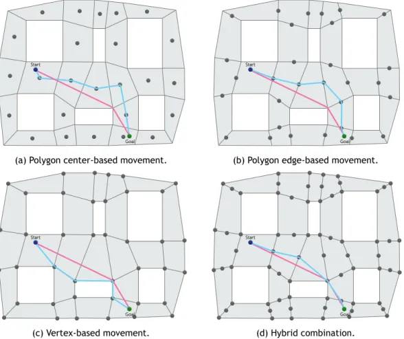
There are many possibilities when trying to navigate through navmeshes, namely polygon center-based movement, edge center-center-based movement, vertex-center-based movement and hybrid combina-tions.

(32)

Polygon center-based movement, as illustrated in Figure 2.6 (a), uses the center of each polygon as a graph node position. Figure 2.6 (b) shows edge center-based movement which consists in moving through the edges between adjacent polygon, where the center of the edges serve as a graph node position. Vertex-based movement, as shown in Figure 2.6 (c), moves through the vertex of the non-defined areas, just like waypoint-based visibility graphs, although this alternative doesn't connect nodes in straight lines. Lastly, a hybrid combination of the previous methods can be employed, as illustrated in Figure 2.6 (d).

(a) Polygon center-based movement. (b) Polygon edge-based movement.

(c) Vertex-based movement. (d) Hybrid combination.

Figure 2.6: Navigational mesh with different node locations.

Figure 2.6 shows the methods described above, where the nodes are represented as grey dots, the blue path is the optimal path, and the pink path is a visually optimal path.

2.4 Search Algorithms

This section describes some of the most known algorithms for pathfinding, in chronological order, Dijkstra's algorithm, A*, Best-first search and Fringe search.

2.4.1 Dijkstra's Algorithm

In 1959, Edsger Dijkstra [Dij59] introduced a method to find the shortest path between two nodes of a weighted graph, where each edge would contain a positive traversal cost. Dijkstra's algorithm is both complete and optimal.

(33)

2.4.1.1 Leading Idea

Dijkstra's algorithm explores the whole graph while keeping track of the cost so far (CFS) value C of each node from the starting node. C values allows to know how far is the currently explored node from the starting node. At each node, the cost to travel to a successor node is added to its C cost. Since multiple paths can exist to a single node, successor nodes may already have a G cost, meaning that there is an existing path to that node, at which point an evaluation of a better path needs to be done. A new C cost is calculated from the current node to the successor node, and in case it has a lower value, the path is updated. This guarantees that the returned path is the shortest path possible, the optimal path.

During the search, Dijkstra's algorithm encounters nodes that fall into different states: unseen, unvisited and visited. When an unseen node is encountered, its C value is calculated. This unseen node now needs to be explored, so it is placed into a list, called the open list, which contains all nodes that need to be explored. A node is removed from the open list in order to be explored, and added to another list, called the closed list, which represents the nodes that have been visited, but visited once. The node popped from the open list to be explored is the node with the lowest C value. This means that it is the node that is closer to the starting node, that is, the shortest path so far. When there are no more nodes in the open list, the algorithm returns the shortest path from the starting node to the goal node.

2.4.1.2 Detailed Description

Dijkstra's algorithm is detailed in Algorithm 1. Dijkstra's algorithm starts by setting the start node's parent reference to null and its C cost to 0 (line 1). The starting node is added to the open list (line 2). For each iteration, while the open list is not empty, the algorithm removes the node with the lowest cost so far value from the open list and sets it to the current node N (lines 3-4). For each successor node S of N, a new cost so far value is calculated, C(s) = C(n) + traversal cost (lines 5-6). Then, if S is unexplored, S's cost so far value is set to the new C(s) value. S's parent is set to N, and S is added to the open list (lines 7-10). If S is in the open list, therefore, explored, and its cost so far value is greater than the new cost so far. S is updated with the new cost so far value, and S's parent reference is set to N (lines 11-13). If S is in the closed list, and S's cost so far value is greater than the new cost so far value. S's cost so far is updated with the new cost so far value. S's parent reference is set to N, and S is removed from the closed list and inserted into the open list (lines 14-18). N is then added to the closed list (line 19). Finally, the algorithm reconstructs the path (line 20).

The memory costs of Dijkstra's algorithm accounts for of the data contained in each node in the graph and the memory costs of the open and closed lists.

Dijkstra's algorithm can still be optimized. At each iteration, since the closest node to the start node is explored, a closer path to a closed node is highly unlikely to be found [Ang12]. Therefore, successor nodes that are already in the closed list can be ignored in the search process, what leads to a more concise algorithm. Removing lines 14 to line 18 from Algorithm 1 would be enough to reflect these changes.

Figure 2.7 shows Dijkstra's search and resulting search space exploration. Bright green node is the starting node, whereas the red node is the goal node. Light blue nodes are explored nodes inserted in the closed list. Light green nodes are called frontier nodes and are seen nodes that

(34)

Algorithm 1 Dijkstra's Search Algorithm 1: Clear start node's parent and C cost.

2: Add start node to open list

3: while open list is not empty do 4: n = best node from open list

5: for all Successor nodes S of n do 6: Calculate new C cost

7: if S is unexplored then 8: Set S's C cost to new C cost

9: Set S's Parent to n

10: Add S to open list

11: else if S is on the open list and S's C cost is greater than new G cost then 12: Set S's C cost to new C cost

14: else if S is on the closed list and S's C cost is greater than new G then 15: Set S's C cost to new C cost

17: Remove S from closed list

19: Add N to closed list

20: Reconstruct path

Figure 2.7: Dijkstra's algorithm search path.

are in the open list, waiting to be explored. Grey nodes represent non-walkable position of the grid map (e.g., walls). The yellow line represents the path from the starting node to the goal node.

2.4.1.3 Point-to-Point Variant

Point-to-point version of Dijkstra's is a variant of Dijkstra's algorithm for video games, since video games usually rely on point-to-point searches (see Figure 2.8). The original version of Dijkstra's algorithm is an all-points search, finding the shortest path from the start node to every single node in the graph. Dijkstra's algorithm explores the entire search space even after it has found the shortest path to the goal. In most cases, this leads to unnecessary computations, and the point-to-point version of Dijkstra's algorithm solves this problem and optimizes it for video games offering significant improvements over the original method [Ang12].

(35)

may exist. This means that if the algorithm terminates as soon as the goal node has been explored, then the current path found to the goal is guaranteed to be the shortest path. This prevents further exploration of the search space. The algorithm remains optimal and complete, while reducing the number of explored nodes, reducing also processing and memory costs and improving search times.

The goal node may be found early on the search, but may not be immediately explored. This is due to other nodes being closer to the starting node than the goal node. In this case, Dijkstra's algorithm will continue the search and explore nodes closer than the starting node postponing the exploration of the goal node. This extra search can be prevented by simply terminating the search as soon as the goal node is found, but this early termination will not guarantee the optimality of the algorithm.

Algorithm 2 shows the improvements made over Dijsktra's original algorithm. Lines 14 to 18 where removed from Algorithm 1 and lines 5 and 6 where added to Algorithm 2. Additions to the algorithm have to do with checking the goal node, when the best node is selected from the open list. In case the node is the goal node, the algorithm reconstructs the path and returns it.

Algorithm 2 Point to Point Dijkstra's Search Algorithm 1: Clear start node's parent and G cost.

5: if n is goal then 6: Reconstruct path

7: for all Successor nodes S of n do 8: Calculate new G cost

9: if S is unexplored then 10: Set S's G cost to new G cost

13: else if S is on the open list and S's G cost is greater than new G cost then 14: Set S's G cost to new G cost

16: Add N to closed list

17: Reconstruct Path

Figure 2.8 shows Dijkstra's point to point search and resulting search space exploration.

(36)

2.4.2 A* Algorithm

The A* algorithm was introduced in 1968 by Peter Hart, Nils Nilson and Bertram Raphael [HNR68] as a variant of Dijkstra's algorithm. However, unlike Dijkstra's algorithm, A* does not ensure that the shortest path is found. Nevertheless, it tends to find the shortest path, using for that the heuristic of the later best-first search [Pea84] (see Section 2.4.3), which directs the search to the goal. A* is one of the most popular search algorithms, not only in games (e.g., pathfinding), but also in other single-agent search problems, such as AI planning, and used to be the de facto standard in pathfinding search. Both the memory and the running time can be important bottlenecks for A*, especially in large search problems [LMP+_{13]. A* returns an optimal solution}

(i.e., admissible) when all cost estimates are not higher than the real cost [DP85].

2.4.2.1 Leading Idea

A* algorithm explores a search graph in a best-first manner, growing an exploration area from the start node until the goal node is found, while remembering the visited nodes, to be able to avoid re-exploration of nodes and to reconstruct a solution path to the goal.

The A* algorithm works by combining the C value used in Dijkstra's algorithm and the heuristic estimate, H, to the goal, into a total estimated cost, referred as F(n) = C(n) + H(n). A* differs from Dijkstra's algorithm on its selection of the node from the open list. Dijkstra's algorithm selects the node that has a lower C value, i.e., the node that is closer to the starting node, while A* selects the node that as a lower F value, which represents the node that has a shorter path so far and that is estimated to be closer to the goal.

2.4.2.2 Detailed Algorithm

A* algorithm, described in algorithm 3, starts by setting the start node values, F, C and H to zero, setting also its parent reference to null (line 1). The start node is added to the open list (line 2). While the open list is not empty, the node with the lowest F value is popped from the open list and is set as the current node (lines 3-4). If the current node is the goal node, the path is returned (lines 5-6). Otherwise, this node is then placed in the closed list as a visited node (line 7). A* checks all neighbors of the current node. For each neighbor N, if S is already in the open list, skip this node (lines 8-10). Otherwise, a tentative C value is calculated as in Dijkstra's algorithm (line 11). Then, if N is not in the open list or its C value is higher than the tentative C value, C value of N is updated with the tentative C value, a new H is calculated, F is updated, and the parent reference is set to the current node (lines 12-15). If S is not in the open list, S is added in the open list for exploration (lines 16-17).

2.4.2.3 Tie Breaking

Upon selection of the next node to retrieve from the open list, it may happen that two or more open nodes may have the same F value but different C and H values. In situations like this, a tie breaking method must be employed. A good tie-break is to use the node with the lowest C value, that would be the node closer to the starting node.

(37)

Algorithm 3 A* Search Algorithm

1: Clear start node's Parent and cost values ( F, C, H )

3: while open list is not empty do 4: n = pop best node from open list

5: if n is goal then 6: Reconstruct path

7: Add n to closed list

8: for all Successor nodes S of n do 9: if S is in open list then 10: continue;

11: Calculate new G cost ( Current C + traversal cost )

12: if S is not in open list or new C cost is lower than S's G cost then 13: Set S's Parent to n

14: Set S's C cost to new C cost

15: Set S's F cost to S's C cost + Heuristic estimate from S to Goal

16: if S is not in open list then 17: Add S into open list

18: Reconstruct No Path

In A* algorithm, node exploration is based on the heuristic value, which is an estimation of the closeness to the goal node. This estimation may often be too optimistic and lead to the exploration of nodes that are farther from the start node before the nodes that are closer to the start node, resulting in the exploration of closed nodes whose C values are overly high and which can still be reduced. This means that closed nodes cannot be ignored as in Dijkstra's algorithm and need to be checked and updated if necessary [Ang12]. Unfortunately, this introduces the concept of re-exploring closed nodes, which does not occur in Dijkstra's algorithm.

Depending on the search problem and search space, the degree of node re-exploration can be quite large. This increases computational cost of A* algorithm, but has no effect on memory cost. Even with this increase in computational cost, total node exploration (i.e., the number of visited nodes) is still significantly less than in Dijkstra's algorithm.

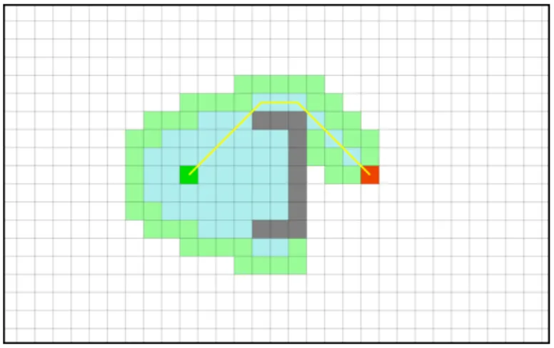
Figure 2.9: A* Algorithm Search Path.

Figure 2.9 shows the search space and resulting path (in yellow) found using A* search algorithm. The bright green node is the starting node, the bright red node is the goal node, the light blue nodes are the visited nodes and the light green nodes are the nodes to be visited, the frontier nodes. The dark grey nodes represent obstacles (i.e., walls).

(38)

2.4.2.4 Heuristics

An heuristics is an estimate of cost incurred in traveling between two nodes. This estimate is given by a function, H(n). The heuristic can alter the search algorithm performance, making it work faster or slower, use more or less memory, be more or less accurate, and optimal or not. In A* algorithm, the next node to explore is chosen based on its associated value, F(n) = C(n) + H(n). Depending on the importance of H(n) over C(n), F(n) will be different, leading to a different path. Some of the possibilities for the importance of different H(n) values are as follows [Pat11] :

• If H(n) is 0, only C(n) will affect on the search resulting the same search result as Dijkstra's algorithm.

• If H(n) is always lower than or equal to the cost of moving from N to the goal, A* is guaranteed to find the shortest path [HNR68]. The lower the estimation, the more nodes A* explores.

• If H(n) is exactly equal to the cost of moving from N to the goal, A* only follows the best path and never explores any other node, making it very fast. Given a perfect heuristic, A* behaves perfectly.

• If H(n) is sometimes higher than the cost of moving from N to the goal, A* will run even faster than using a perfect heuristic, but there is no guarantee to find an optimal path.

• If H(n) is very high relatively to C(n). In this case, only H(n) affects the search. This returns the same search result as the best-first search.

A* can be fine tuned towards speed or accuracy depending on the needs of the search algorithm. In many video games a "good enough" path may be sufficient and by raising the estimation, the search will run faster, returning a nearly optimal path. On the other hand, when the estimation is lower or exact, a more accurate and slower search will return an optimal path from N to the goal.

The balance between accuracy and speed can be regulated dynamically in-game. By giving a weight to the heuristic cost, the algorithm is able to control how accurate the search needs to be. On a large search area, A* may be tuned to run faster on the hope that the path may be re-calculated with more accuracy when closer to the goal. This way, the slower search will run closer to the goal with a reduced search space leading to an equally fast search without loosing performance or path quality.

Note that C(n) and H(n) must have the same scale in order to ensure that the algorithm behaves correctly. For example, if C(n) returns values in meters and H(n) in kilometers, H(n) will clearly have much more influence on the resulting value F(n).

A number of well known heuristics have been used in A* algorithm. In a plane, with standard coordinates Aiand Bi, respectively, heuristics are:

(39)

plane, the Euclidean distance is defined as: Deuclidian(A, B) = v u u t∑n i=1 (Ai− Bi)2 (2.1)

• The Manhattan distance [Bla06] is the distance between two points measured along axes at right angles. In a plane, the Manhattan distance is defined as:

Dmanhattan(A, B) =

k

∑

i=1

|Ai− Bi| (2.2)

• The Chebyshev distance [Bla08], also known as maximum metric, is the greatest difference between two points. In a plane, the Chebyshev distance is defined as:

Dchebyshev(A, B) = max (|Ax− Bx| , |Ay− By|) (2.3)

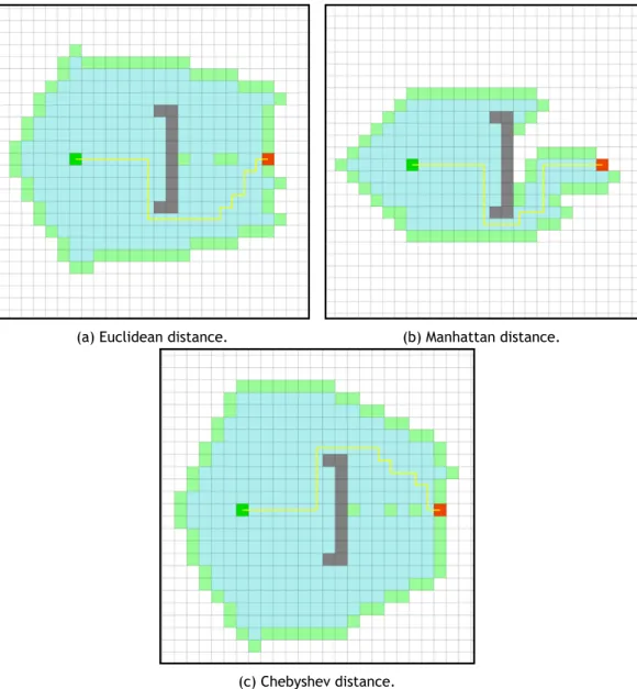
(a) Euclidean distance. (b) Manhattan distance.

(c) Chebyshev distance.

Figure 2.10: A* search path results using different heuristics.

(40)

Eu-clidean distance uses the square root operation which will reduce performance and should be avoided when possible. Using the euclidean distance, H(n) will have lower values than Manhat-tan's or Chebyshev's distances, making the cost function C(n) not match the heuristics. Heuristics that do not over-estimate the true distance to a goal node are said admissible. A* with an ad-missible heuristic returns optimal solutions [HNR68]. Figure 2.10 (b) shows A* algorithm's search path in a 4-connected grid using the Manhattan distance as the heuristic. Figure 2.10 (c) shows the resulting path of A* search algorithm using Chebyshev distance. Light green nodes are the frontier nodes, which are the nodes on the open list. Light blue squares are the visited nodes. Green is the starting node and red the goal node. Grey nodes represent non-passable nodes (e.g., walls).

Each of these heuristic costs are multiplied by a distance cost, D, which is based on the lowest cost between two adjacent nodes. In the absence of obstacles and terrains that have a minimum cost D, moving to a step closer to the goal should increase C(n) by D and decrease H(n) by D. When adding the two components C(n) and H(n), F(n) remains the same, meaning that the heuristic and cost function scales are a match. On the other hand, if the scales do not match, then either the heuristic or the cost function has too much weight on the final calculation [Pat11].

Figure 2.10 shows different search areas of exploration using different heuristics. With the same search map and same search algorithm applied, all of the heuristics returned a path length of 26 nodes, which is the optimal path. Using the Manhattan distance, however, leads to end the algorithm in 331 steps, whereas Euclidean distance takes 566 steps to finish and Chebyshev distance 648 steps. Figure 2.10 clearly shows the increase in nodes explored justifying the results obtained.

2.4.2.5 A* Variants

Over the years A* suffered many alterations in order to correct some aspects of the algorithm and to fulfill the needs of ever demanding commercial games, what gave birth to not only new algorithms such as Iterative Deepening A* (IDA*) [Kor85], Memory Enhanced IDA* [RM94], Fringe Search [Bjo05] but also new paradigms of pathfinding with hierarchical abstractions on grid maps and parallel searches.

IDA* [Kor85] is a depth-first search algorithm and works by searching the graph depth by depth via a threshold factor on the F(n) value. When F(n) is too large, the nodes are not be considered. At the beginning, IDA* expands a few nodes and at each subsequent iteration, the number of visited nodes increases. If a better path is found, the threshold is increased. IDA* revisits nodes when there are multiple, possibly non-optimal, paths to a goal node, which is often solved by using a transposition table as a cache of visited nodes [RM94]. When using a cache of visited nodes, IDA* is denoted as memory-enhanced IDA* (ME-IDA*). IDA* repeats all previous operations in a search when it iterates on a new threshold, what is necessary to operate when no storage is used. By storing the leaf nodes of a previous iteration and using them as the starting position of the next, IDA* efficiency improves significantly. These improvements gave birth to the fringe search algorithm [Bjo05], which is described in Section 2.4.4.

Weighted A* [Poh70] also provides significant speed-up at the price of a bounded solution sub-optimality [LMP+_{13]. There are many other search methods that build on A*, including methods}

for hierarchical pathfinding, such as, Hierarchical Pathfinding A* (HPA*) [BMS04], Hierarchical Annotated A* (HAA*) [SSGF11], Partial Refinement A* (PRA*) [SB05], Block A* [YBHS11] and

(41)

meth-ods for search on multiple CPU (Parallel Ripple Search [BB11]) [LMP+_13].

2.4.3 Best-First Search

2.4.3.1 Leading Idea

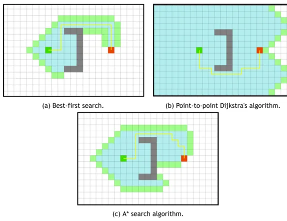
Best-first search [Pea84] is a greedy algorithm that was inspired by A*, but only uses a heuristic to guide the search to the goal, not using the cost so far. Consequently, best-first search con-verges to the goal faster and explores a smaller amount of nodes, as illustrated in Figure 2.11a. However, best-first search does not guarantee to find the shortest path neither the optimal path as A*.

The main disadvantage of best-first search is that it is a greedy algorithm. A greedy algorithm will direct the search to local minima fairly easily, since it only considers the estimate value to the goal node, causing the exploration of nodes even when the search is not on the right path. The lack of knowledge on the traveled path so far may lead to long, non-optimal paths.

(a) Best-first search. (b) Point-to-point Dijkstra's algorithm.

(c) A* search algorithm.

Figure 2.11: Search space explication comparison.

Figure 2.11 compares the different algorithm search results and search space explorations.

The best-first search also works with an open list and a closed list (see Algorithm 4). Best-first search starts by adding the start node to the open list (line 1). At each iteration, while the open list is not empty, the node with the lowest F(n) value, defined by F(n) = H(n), from the list is popped out and set as the current node (lines 2-3). If the current node is the goal, the algorithm

(42)

returns the reconstructed path (lines 4-5). At this point, every neighbor of the current node is examined, added to the open list and their parent's reference is set to the current node (lines 6-9).

Algorithm 4 Best-First Search 1: push start node to open list

4: if goal is found then 5: Reconstruct path

6: for all neighbor S in n do 7: Explore S

8: Push S into open list

9: Set S's parent to n

2.4.4 Fringe Search Algorithm

2.4.4.1 Leading Idea

Fringe search algorithm [Bjo05] can be seen as a variant of A* or a variant of IDA*. As mentioned in Section 2.4.2.5, IDA* disadvantages are solved through the inclusion of cache memory to avoid repeated states and the now list and after list to remove unnecessary iterations over the same nodes, give birth to the fringe search algorithm.

Considering how IDA* works, there is a starting threshold H (root). The algorithm does a recursive left-to-right depth-first search, so that the recursion stops when either a goal is found or a node is reached that has an f value bigger than the threshold. If the search with the given threshold does not find a goal node, the threshold is increased and another search is performed.

As said above, Fringe search uses two lists, the now list and the later list (see Algorithm 5). At each iteration, the leaf nodes are added to the later list to be explored in the next iteration. When the iteration completes, the later list becomes the now list, and when a new iteration begins, the search will resume from the now list, instead of re-iterating over the whole search tree. Fringe search algorithm does not need to keep the later list and now list ordered when compared to A*, which leads to improved computational costs. However, fringe search algorithm will revisit nodes. Fringe search explores on the limits of the graph, hence the term, fringe.

2.4.4.3 Algorithm

2.5 Final Remarks

Grid-based map representations (discussed in Section 2.3) have several drawbacks that may make them less useful in games in which environment objects don't have uniform sizes or shapes

(43)

Algorithm 5 Fringe Search Algorithm 1: fringe F = s

2: cache C[start] = (0, null)

3: found = false

4: while (found is false) AND (F not empty) do 5: fmin = ∞

6: for all N in F, from left to right do 7: (g, parent) = C[node]

8: f = g + h(node)

9: if f is greater than flimit then 10: fmin = min(f, fmin)

11: Continue

12: if node is goal then 13: found = true

14: break

15: for all child in children(node), from left to right do 16: child g = g + cost(node, child)

17: if C[child] is not null then 18: (g cached, parent) = C[child]

19: if g child is greater than or equal to g cached then 20: Continue

21: if child in F then 22: Remove child from F

23: C[child] = (g child, node)

24: Remove node from F

25: flimit = fmin

26: if reachedgoal is true then 27: Reconstruct path

and where large areas of the map are empty leading to a waste of space [LMP+_{13]. Demyen}

and Buro [DB06] present two pathfinding algorithms to address these problems, Triangulations A* (TA*), and Triangulation Reduction A* (TRA*). TA* uses dynamic constrained Delaunay triangu-lations (DCDT [KBT04]) to represent maps in which obstacles are defined by polygons, and finds optimal any-angle paths for circular objects by running an A* like algorithm on graphs induced by the triangulation.

Dijkstra's algorithm was designed to be a all-point search, finding all paths from a single node in a graph, exploring the entire graph. This leads to a very high computational cost, estimated around O(n2₎_{where "n" is the number of nodes in the graph. Processing costs are a result of}

operations on open and closed lists. Each time a node is selected from the open list, the entire list is searched to find the node with the lowest G value. With each node explored, the open list grows in size and so the cost of performing this search. The open list search is the most computationally expensive operation in the algorithm and therefore has been a primary focus for optimization for both Dijkstra's algorithm and algorithms derived from it, such as A* and its variants.

A simple way of reducing the open list searching costs is to store the nodes in an ordered manner. If the open list is ordered in ascending order, the first node will always be the best node. Selecting the best node from the list becomes a trivial operation with respect to processing costs. Unfortunately, keeping the list ordered introduces additional costs during node exploration. When a node is inserted into the list, a search done to find the correct position to insert the node. When a node is updated, its C(n) or F(n) cost, depending on the algorithm used, will change and the node will change position inside the list, leading to extra operations by removing

(44)

and re-inserting the node into the list.

The closed list serves the purpose of checking whether a node has been visited or not. When examining successor nodes, a verification is done to verify if the node has already been visited, which would be indicated by being present in the closed list. When the closed list grows in size, searching for a particular node becomes quickly expensive. A simple solution around this issue is to have the nodes carrying a search state flag indicating whether they are unseen, unvisited or visited. When examining the nodes, changing its search state flag instead of inserting and removing it from lists allows the algorithms to perform better, both in time and memory. The closed list becomes obsolete and can be completely removed from the algorithm.

Uniform travel cost on maps lead to a considerable degree of symmetry in a pathfinding prob-lem [LMP+_{13]. Symmetry reduction is based on empty rectangles identified on a map [HB10]}

[HBK11]. Given two nodes A and B on the border of an empty rectangle, all optimal paths con-necting these are symmetrical to each other, and considering only one such a path is sufficient. Jump Point search [HG11] takes a different approach to symmetry elimination. It allows prun-ing part of the successors of a node, ensurprun-ing that optimality and completeness are preserved [LMP+_13].

(45)

Chapter 3

Influence Map-Based Pathfinding

Real-time strategy (RTS) games are a sub-genre of strategy games in which a player interacts in real time without awaiting for another player's turn [Bur03] [BF03]. RTS games such as for example, Starcraft by Blizzard Entertainment [Ent] and Age of Empires by Ensemble Studios [Stu] are usually set on a war theme [SDZ09] and require the player to gather resources, perform base management, unit coordination, and defeat enemies in real time [BF03].

In RTS games, all player's decisions are taken independently of other players, with no need to wait for a player's turn to finish [HJ08]. RTS games often require the player to control a great amount of units (i.e., troops, vehicles, planes, etc.) that is, units in movement. This movement of game units poses a challenge to pathfinding in games. In fact, pathfinding methods for these units may become slow when one need to calculate similar paths for hundreds of units that move in groups to the same location. To prevent these intensive calculations, one uses potential fields in path planning. Pathfinding specifically applied to the RTS genre focuses on alternatives, such as path planning using potential fields [BK89] [Bur03].

3.1 Potential Fields

One cannot talk about influence maps before first talking about potential fields. Potential fields (PF) or artificial potential fields (APF) are a technique used to avoid collisions and achieve human like movement of game agents in real-time [Joh12]. The leading idea of potential fields has some similarities with influence maps further discussed in Section 3.2. In 1985, Ossama Khatib came up with the idea of artificial potential fields in robotics, as a way to avoid obstacles and achieve human like movements [Kha86]. Later, Arkin proposed a new technique based on spatial navigation of vector fields that proved to be better than previous methods [Ark97]. The game's efficiency regarding object movement can be increased by applying different types of potential fields, simultaneously [HJ08] [HJ09a] [HJ09b].

3.1.1 Overview

Potential fields work by strategically placing attractive and repulsive force propagators in the game world. A propagator is a game unit that delivers a potential field. In fact, a propagator generates a potential field that gradually fades to zero [Hag08]. Generally, if its charge is attractive, other objects move towards it, if its charge is repulsive other objects move away from it.

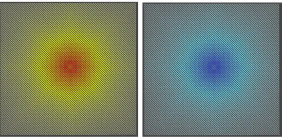
Figure 3.1 (a) represents an attractive propagator, where the field of forces are represented by a vector field. Figure 3.1 (b) shows the repulsive potential field. The attractive field is uniform throughout the map, but fades near the propagator. The same does not happen with repulsive

(46)

(a) Attractive Potential Field (b) Repulsive Potential Field

Figure 3.1: Attractive and repulsive force fields.

fields. Repulsive forces decay with distance to the propagator, having a higher force near the propagator. The origin of either potential field is the position of the propagator.

(a) Resulting potential field of two charges.

(b) Resulting possible path from agent.

Figure 3.2: Opposing charges in same potential fields.

As illustrated in Figure 3.2 (a) and Figure 3.2 (b), the potential field spreads over the totality of the map. The attractive forces are present in most parts of the map, while the repulsive force change the attractive forces, and ultimately change the direction and intensity of the field near the repulsive propagators. Figure 3.2 (b) shows a possible path taken from an agent, which avoids the repulsive charge and continues to navigate to the goal.

3.1.2 Potential Field Types

There are two major types of potential fields namely: point fields and directional fields. The point fields converge/diverge to/from a point located at a finite distance. The directional fields assume that the propagator is in the infinite. There are three categories of point fields: attractive, repulsive, attractive-repulsive and two categories of directional fields: uniform, perpendicular.

(47)

Attractive potential fields, as illustrated in Figure 3.1 (a), are used to represent the goal or any important location, and are used to lure the agents to their center [Hag08]. Repulsive potential fields, shown in Figure 3.1 (b), are the opposite of attractive potential fields, which pushes away agents from a game world zone, obstacles, or units [Hag08] so they can avoid each other.

Figure 3.3: Asymmetric Potential Field. The path avoids facing the turret [SuI11].

Asymmetric potential fields, as illustrated in Figure 3.3, can have both attractive and repulsive forces coming from the same object. Figure 3.3 shows an example of a asymmetric potential field generated by a turret [SuI11]. This is useful when the agents need to act according to a strategy (e.g., flank the enemy). This way, the agent will not face the turret and risk being hit, instead, it will try to flank it and reach it from behind.

(a) Uniform potential field [SuI11]. (b) Perpendicular potential field [SuI11].

Figure 3.4: Different types of potential fields.

Uniform potential fields, shown in Figure 3.4 (a), guide agents in a specific direction and will not be able to guide them to the goal but are good at following walls [Goo10]. Perpendicular potential fields, shown in Figure 3.4 (b), are used to guide the agent away from a wall [Goo10].

3.1.3 Local Minima

Local minima likely is the most important problem that we find in artificial potential fields. Figure 3.5 shows an example of an agent stuck at a local minimum. If the goal is on the other side of the wall, the agent cannot go further, because the total sum of vector forces reaches zero, having no force nor direction to proceed any further.

One solution is to apply a random potential field to get the agent out of the local minimum [Goo10]. Another solution, as proposed by T. Laue [TL03], is to apply A* pathfinding search to find a suitable location to resume motion planning using potential fields when such location is reached. In short, in this scenario, A* is used to solve local minimum situations exclusively,

(48)

Figure 3.5: Local minima problem with U-shaped obstacle.

otherwise, one uses potential fields. That is, in the current state-of-the-art, A* and potential fields are never ran simultaneously.

In contrast, this dissertation is entirely based on combining existing search algorithms (i.e., Di-jkstra's, A*) with the spatial reasoning provided by influence maps, in order to make pathfinding searches reactive to their environment (i.e., given updated information of the game environ-ment changes), and find solutions faster (i.e., searching less nodes).

Yet, another solution is to avoid returning to the previous position in the potential field, as proposed by T. Balch and R. Arkin [TR93]. The solution consists in releasing repulsing potential force at regular intervals. To reduce interference with goal based potential fields, Thurau et al. [CTS04] proposed that the avoid-past potential field forces are reduced over time, resulting in a pheromone trail effect known from ant-algorithms. The pheromone-like repulsive potential forces push the agent from nearby nodes to avoid local minima.

3.2 Influence Maps

Influence maps evolved from work done on spatial reasoning for the GO game [Zob69]. Spatial and temporal reasoning has to do with the analysis of terrain as well as understanding events that occur over time. Influence maps have been used in video games [Toz01], more specifically for games such as Ms. PacMan [WG08] [SJ12], real-time strategy games [ML06a] [ML06b] [MQLL07] [Mil07] and turn based games [LM05].

Influence maps introduce two concepts into spatial reasoning: tactics and strategy. Tactics is a word from ancient Greek that means art of arrangement, which is used to refer specific actions or specific tasks by game agents; for instance, where a player should place a defense tower. Strategy is referred to high level planning to achieve goals under unknown conditions (i.e., adversarial troops, enemy location), which will impact the outcome of the game.

There are many possible representations for tactics information, such as artificial neural net-works and knowledge based approaches. However, Avery et al. [ALA09] used influence maps due to their intuitive representation of spatial characteristics of game worlds.

(49)

(a) Influence map over game world. (b) Top view of influence map over game world.

Figure 3.6: Influence map representations over a game world.

Strategy is used to make high-level decisions, namely, deciding which town to conquer next and why (i.e., precious resource). Tactics are used to make low-level decisions, at the game agent level, namely to decide which path to take, which enemy faction to attack and why (i.e., shortest path, weaker enemy). Influence maps provide information for both tactical and strategic decision making [Swe06].

Influence maps allow intelligent inferences about the game environment, namely, where the enemy has less troops, which country to invade, or other meaningful information that human players inherently would perceive through experience and intuition [Toz01] [WG00].

3.2.1 Overview

Similarly to potential fields (see section 3.1), influence maps have propagators carrying positive or negative influence. The main difference between potential field and influence maps is how the propagation is done. Whereas potential fields generate vector fields of forces, influence maps produce scalar fields of influence.

Figure 3.7: Visual representation of influence values.

(50)

at the center of the influence are the source of the propagators. From there, the influence looses force and gradually fades to zero. The values range from 10 to 0 and -10 to 0, for an easy visualization and representation purposes only.

Repulsive and attractive propagators may carry negative or positive scalar values, which depends on implementation. On the contrary, from here on now, we assume that repulsive propagators carry a positive value and attractive propagators carry a negative value. As usual, propagators can be game units, game events, or any other game entity, as long as they are located in the game environment space.

(a) Repulsive propagator. (b) Atractive propagator.

Figure 3.8: Repulsive and attractive propagators.

Figure 3.8 (a) shows a repulsive propagator carrying positive influence value, while Figure 3.8 (b) illustrates an attractive propagator carrying negative influence value. The darker colors at the center of the propagator represents the epicenter of the influence propagation, which is a minimum for attractive propagator and a maximum for repulsive propagator, fading gradually outwards to zero.

As discussed in Section 2.3, 2D grid-based representations are relatively easy to use and im-plement. Influence maps can be represented by 2D grids and also abstracted into 3D influence volumes [Pot00]. Influence map representation is overlapped on top of the game environment. Influence maps can be layered to create new information by merging different influence map information, e.g., faction influence, town control influence, combat strength, visibility area, noise, frontier of war, unexplored areas, recent combats, and more [Toz01] [WG00].

Tozour [Toz04] proposed an approach in which each influence map layer, representing distinct information, are merged into a final influence map as a weighted sum, in which the weights are chosen arbitrarily.

Bergsma et al. [BS08] used a neural network (NN) for a layering algorithm to generate two influence maps, one indicating the trend of moving to a tile and the other indicating the trend of attacking a tile. Both influence maps are merged to maximize chances of moving and attacking a tile. Sweetser [Swe04] also used neural network and influence maps for strategic decision-making in games.

(51)

(a) Negative and positive influence at opposing sides.

(b) Random influence propagation outcome.

Figure 3.9: Posible final influence map representation.

how the influence propagates with randomly set propagators.

Influence maps are also used in non-violent game scenarios. Sim City [sim] series offer real-time maps that show the influence of police and fire departments around the city. These influence maps are used by the player, so high-level strategic decisions can be made, for instance, placing a police building that will help cover zones where there is low police influence.

Influence maps help the artificial intelligence to make better decisions, given useful information about the game world. They provide three types of information that are particularly useful for decision making [Cha11] namely:

• Situation Summary: Influence maps summarize the details in the world making them easy to understand at a glance. This is so because they provide visual feedback about where the influence is, who is in control of an area, and so on, are procedures that becomes trivial.

• Historical Statistics: Influence maps hold information for a limited amount of time, al-lowing the temporal analysis of recent events (i.e., recent war zones). This is controlled with the momentum parameter (see Section 3.2.3.1).

• Future Predictions: Influence maps predict upcoming events [LMAB+_{09]. Using terrain}

maps, enemy influence can be analyzed to know where they are headed.

On large and open game environments that have varying traversal costs between nodes, choke-points and large obstacles, influence maps provide interesting properties to help the game AI make better decisions, due to how the propagators influence is spread against with each other [Cha11].

3.2.2 Representations

Similarly to any game environment, influence maps needs to have two main components to be able to be represented, namely: spatial partitioning and connectivity.

Influence map-based pathfinding algorithms in video games

Engenharia

Influence Map-Based Pathfinding Algorithms in

Video Games

Michaël Carlos Gonçalves Adaixo

Dissertação para obtenção do Grau de Mestre em

Engenharia Informática

(2º ciclo de estudos)

Orientador: Prof. Doutor Abel João Padrão Gomes

Acknowledgments

Resumo

Palavras-chave

Abstract

Keywords

Contents

List of Figures

List of Tables

Acronyms

Chapter 1

Introduction

1.1

Motivation

1.2

Problem Statement

1.3

Scheduling of the Research Work

1.4

Contributions

1.5

Organization of the Thesis

1.6

Target Audience

Chapter 2

State-of-the-Art in Pathfinding

2.1

Introduction

2.2

Pathfinding

2.3

Search Space Representation

2.3.1

Grid-based

2.3.2

Waypoint-based

2.3.3

Mesh-based

2.4

Search Algorithms

2.4.1

Dijkstra's Algorithm

2.4.2

A* Algorithm

2.4.3

Best-First Search

2.4.4

Fringe Search Algorithm

2.5

Final Remarks

Chapter 3

Influence Map-Based Pathfinding

3.1

Potential Fields

3.1.1

Overview

3.1.2

Potential Field Types

3.1.3

Local Minima

3.2

Influence Maps

3.2.1

Overview

3.2.2

Representations