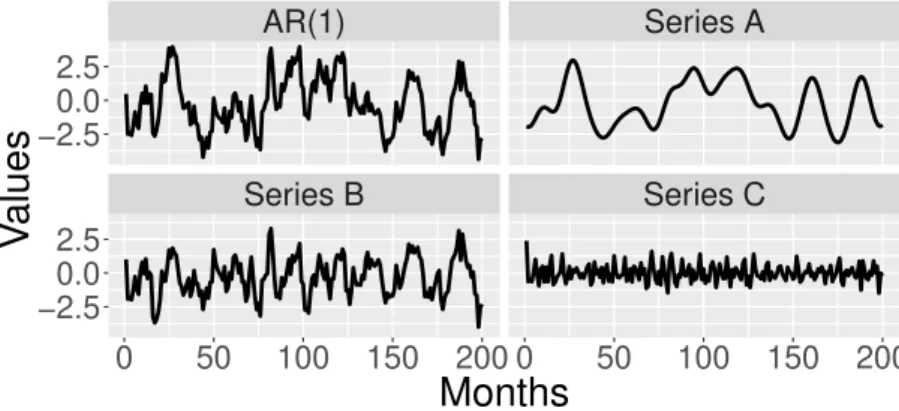
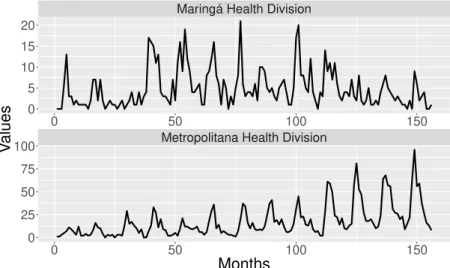
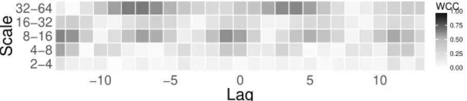
Wavelet Cross-correlation in Bivariate Time-Series Analysis

Apresenta-se nesta seção, uma síntese dos principais resultados levantados de forma a situar o leitor. Em relação ao objetivo “a) Caracterizar os projetos de extensão

Ao Dr Oliver Duenisch pelos contatos feitos e orientação de língua estrangeira Ao Dr Agenor Maccari pela ajuda na viabilização da área do experimento de campo Ao Dr Rudi Arno

Neste trabalho o objetivo central foi a ampliação e adequação do procedimento e programa computacional baseado no programa comercial MSC.PATRAN, para a geração automática de modelos

Ousasse apontar algumas hipóteses para a solução desse problema público a partir do exposto dos autores usados como base para fundamentação teórica, da análise dos dados

Verificamos que muitos pesquisadores apontam para essa problemática e indicam que os professores do ensino regular não possuem formação adequada para atender à proposta da

Conheceremos nesta unidade os tipos de modais, suas infraestruturas, seus riscos, suas vantagens e desvantagens, assim como o papel da embalagem e da unitização para redução

gulbenkian música mecenas estágios gulbenkian para orquestra mecenas música de câmara mecenas concertos de domingo mecenas ciclo piano mecenas coro gulbenkian. FUNDAÇÃO

Para a elaboração deste trabalho, utilizou-se das seguintes estratégias de coleta de dados: descrição da experiência profissional do autor; análise da estrutura física da