Causal Nexus Between Economic Growth, Inflation, Stock Market Development and Banking Sector Development

(1)

UNIVERSIDADE DA BEIRA INTERIOR

Ciências Sociais e Humanas

Causal Nexus Between Economic Growth,

Inflation, Stock Market Development and Banking

Sector Development: A Panel-VAR Approach for

High Income Countries

Pedro Nuno Pinheiro Gaiolas

Dissertação para obtenção do Grau de Mestre em

Economia

(2º Ciclo de Estudos)

Orientador: Prof. Doutor José Alberto Serra Ferreira Rodrigues Fuinhas

(2)

(3)

i

Acknowledgments

I wish to thank, in first place, to Professor José Alberto Fuinhas for sharing expertise and for having accepted my invitation to be my supervisor. I couldn’t be here if it wasn’t for him and for that, I am truly grateful.

I also thank my family, especially my parents, and friends for never letting me give up and for the support they gave me during this challenge.

Finally, my sincerely thanks to all the colleagues that helped with my difficulties along the way. Without them, it would be much harder to succeed.

(4)

(5)

iii

Resumo

A relação entre crescimento económico, inflação, desenvolvimento do mercado de ações e desenvolvimento do setor bancário foi estudada num painel de 21 países de rendimento elevado classificados pelo World Bank para o período 2001-2014 usando dados anuais. Todos os dados usados são extraídos do World Development Indicators do World Bank. Foi usando o PIB per capita constante para estudar o crescimento económico, a inflação no final do período para estudar a inflação e foi usado análise de componentes principais para a construção de duas variáveis que permitem o estudo do desenvolvimento do mercado de ações e do desenvolvimento do setor bancário, num painel VAR, testando a interdependência entre as variáveis bem como a causalidade à Granger, encontrando a presença de tanto causalidade unidirecional como bidirecional entre as variáveis. São também usadas as funções impulso-resposta e a decomposição da variância. Esta investigação defende que o desenvolvimento do mercado de ações e o desenvolvimento do setor bancário estimulam a economia.

Palavras-chave

Painel VAR; crescimento económico; inflação; desenvolvimento mercado de ações; desenvolvimento do setor bancário; análise de componentes principais

(6)

(7)

v

Resumo alargado

A relação de causalidade entre o crescimento económico, a inflação e o desenvolvimento financeiro tem sido amplamente estudado na comunidade científica. Os primeiros trabalhos na área da relação finanças-crescimento defendiam um papel positivo do desenvolvimento financeiro no crescimento económico. Desde o trabalho Schumpeter (1911), foram feitos mais estudos científicos sobre esta relação causal e muitos apresentam resultados diferentes entre si devido a diferentes metodologias aplicadas, países, variáveis e horizonte temporal. Muitos estudos têm demonstrado que existe uma relação positiva de longo prazo entre o desenvolvimento financeiro e o crescimento económico, o que sugere que um sistema financeiro bem desenvolvido é um mecanismo que impulsiona o crescimento económico. Pelo contrário, países com desenvolvimento financeiro menor terão mais dificuldades em estimular o crescimento económico. No estudo de Fung (2009), é reforçada esta ideia ao concluir que países com fraco desenvolvimento financeiro estão presos num círculo vicioso no qual o fraco desenvolvimento financeiro leva a um fraco crescimento económico.

Uma das grandes questões que os investigadores enfrentam nesta área é como é que o desenvolvimento financeiro guia o crescimento económico. Neste sentido, 4 hipóteses são mencionadas na literatura relativamente à direção da causalidade entre variáveis: hipótese neutra, onde não existe qualquer tipo de relação causal entre as variáveis; hipótese

supply-leading e demand-following, onde existe causalidade unidirecional entre as variáveis e,

finalmente, a hipótese feedback, onde existe causalidade bidirecional entre as variáveis. Nesta dissertação é estudada a relação causal entre o crescimento económico, a inflação e duas subcomponentes do desenvolvimento financeiro: o desenvolvimento do mercado de ações e o desenvolvimento do setor bancário. Estas variáveis são estudadas num painel de 21 países de rendimento elevado classificados pelo World Bank num horizonte temporal de 2001 a 2014 usando dados anuais. Todos os dados são extraídos do World Bank e do Fundo Monetário Internacional. Para estudar o crescimento económico, a proxy escolhida foi o PIB per capita constante a preços de 2010, para estudar a inflação foi usada a inflação no fim do período e para estudar o desenvolvimento do mercado de ações e o desenvolvimento do setor bancário foi usado o PCA para, através de várias variáveis, criar uma única que permita avaliar o desenvolvimento do mercado de ações e outra que permita avaliar o desenvolvimento do setor bancário. Para avaliar a adequabilidade do PCA com as variáveis usadas usou-se o teste de adequabilidade de Kaiser-Meyer-Olkin assim como o teste de Bartlett. São efetuados ainda testes preliminares às variáveis tais como o teste VIF para testar a multicolinearidade entre variáveis, teste Hausman para testar se o painel é de efeitos fixos ou aleatórios e o teste Pesaran para testar a dependência seccional (cross section dependence

)

.

(8)

vi O modelo aplicado é um PVAR (painel vetor autorregressivo) desenvolvido por Love & Zicchino (2006) onde todas as variáveis são tratadas como endógenas. O estimador usado é o do Método Generalizado dos Momentos (GMM); é usado o teste de Granger para analisar a causalidade entre as variáveis; a decomposição da variância que mostra a percentagem da variação de uma variável que é explicada pelo choque noutra variável que acumula ao longo do tempo; as funções impulso-resposta que mostra através de gráficos os choques das variáveis em resposta a outras variáveis e o teste de estabilidade do PVAR, mostrando através de um círculo de raio 1, os eigenvalues que são mostrados através de pontos e os quais têm de se situar dentro do círculo.

Nesta dissertação são encontradas relações de causalidade bidirecional entre várias variáveis, assim como causalidade unidirecional entre a inflação e o desenvolvimento do setor bancário e entre o desenvolvimento do mercado de ações e o desenvolvimento do setor bancário confirmando tanto a teoria feedback como a teoria supply-leading, o que vem em linha com alguns estudos referenciados na revisão da literatura. As funções impulso-resposta mostram também que estas variáveis estabilizam num período máximo de 5 anos e que existe uma relação positiva entre o desenvolvimento do sistema bancário e o crescimento económico e entre o desenvolvimento do mercado de ações e o crescimento económico confirmando o que muitos autores concluíram nos seus trabalhos sobre a relação desenvolvimento do sistema financeiro-crescimento económico.

(9)

(10)

viii

Abstract

The relationship between economic growth, inflation, stock market development and banking sector development was studied in a panel of 21 high income countries classified by the World Bank for the period 2001-2014 by using annual data. All the data used is from the World Development Indicators. It was used Gross Domestic Product per capita constant in order to study economic growth, inflation at the end of period to study inflation and it was used principal component analysis for the construction of two single variables that allows the assessment of stock market development and banking sector development in a panel vector auto-regressive model, for testing the interdependence between variables as well as the Granger causalities, finding the presence of both unidirectional and bidirectional causality links among them. It is also used impulse response functions and variance decomposition. The research supports that the stock market development and the banking sector development stimulates economic growth.

Keywords

Panel VAR; economic growth; inflation; stock market development; banking sector development; principal component analysis

(11)

(12)

x

Figures List

Figure 1. Impulse-response functions Page 12 Figure 2. Eigenvalue stability condition Page 13

(15)

(16)

xiv

Tables List

Table 1. Studies confirming the neutral hypothesis

Page 3 Table 2. Studies confirming the supply-leading

hypothesis

Page 3 Table 3. Studies confirming the

demand-following hypothesis

Page 4 Table 4. Studies confirming the feedback

hypothesis

Page 4 Table 5. Variables description Page 5 Table 6. Bartlett test of sphericity and

Kaiser-Meyer-Olkin Measure of Sampling Adequacy for the construction of SMD

Page 6

Table 7. Bartlett test of sphericity and Kaiser-Meyer-Olkin Measure of Sampling Adequacy for the construction of BSD

Page 6

Table 8. VIF test Page 8

Table 9. Pesaran CD-test Page 8

Table 10. Hausman test Page 9

Table 11. Lag order selection Page 9

Table 12. VAR model results Page 10

Table 13. Granger causality test Page 11 Table 14. Forecast-error variance decomposition Page 13

(17)

(18)

xvi

Acronyms List

GDP - gross domestic product PCA - principal component analysis INF - inflation

SMD - stock market development BSD - banking sector development PVAR - panel vector auto-regressive GMM - generalized method of moments VIF - variance inflation test

(19)

(20)

1

1. Introduction

The relationship between economic growth, inflation, stock market development and banking sector development has been widely studied among the scientific community. The academic research on the finance-growth nexus dates to Schumpeter (1911) who defended the positive role of financial development on economic growth. However, the relationship between financial development and economic growth studies have presented us with different results due to different methodologies, countries and time span. One of the big questions in the literature is how the finance guides the economic growth. Hence, 4 hypotheses are mentioned by researchers regarding the direction of causality between the variables: null hypothesis, supply-leading hypothesis, demand-following hypothesis and feedback hypothesis.

In the last decade’s most countries have adopted new development strategies that prioritize the modernization of their financial sector and the link of that sector to economic growth. Clearly, financial development is a matter of considerable policy relevance, especially for major economies that have recently been taking steps to open their capital (Pradhan et al., 2017). In the literature, the financial sector development is disaggregated into various sub-sections but this paper only focuses on two: stock market development and banking sector development. The level of banking sector development and stock market development is among the most important variables identified by the empirical economic growth literature as being correlated with economic growth performance across countries (Fink et al., 2009).

Using a panel vector auto-regressive model to capture not only Granger causality among variables, but also impulse-response functions and variance decomposition to see the shocks variables suffer in a certain time interval. To try to capture economic growth it is used real Gross Domestic Product per capita. Regarding other variables, it is used inflation at the end of period to study inflation and it is used principal component analysis (PCA) to create two single variables to assess stock market development and banking sector development. These variables are studied in the context of high income countries as so classified by the World Bank for the period 2001-2014. Results of this study allows us to better understand how financial development (namely stock market development and banking sector development) impacts economic growth in some major economies.

This paper evolves as follows. Section 2 covers the literature review, Section 3 covers the data and methodology, Section 4 shows the preliminary tests, Section 5 shows the empirical results and finally on Section 6, the concluding remarks.

(21)

2

2. Literature Review

The causal nexus between economic growth, inflation, stock market development and banking sector development has been object of study in the last decades. These studies’ goal is to assess the role inflation, stock market development and banking sector development have on economic growth. Since the work of Schumpeter, many researchers have studied the impact financial sector development has on economic growth and due to different methodologies, data, variables and time span these studies present us with heterogenic results.

The financial sector development was studied by Pradhan et al. (2017) whom disaggregated it into four sub-categories: banking sector development, stock market development, bond market development and insurance market development. Many authors follow this line of work by studying financial development with these four sub-categories. However, this paper only focuses on two: the banking sector development and the stock market development.

The level of banking sector development and stock market development is among the most important variables identified by the literature as being correlated with growth performance across countries (e.g. Levine and Zervos, 1998; Garcia & Liu, 1999; Beck & Levine, 2004; Naceur & Ghazouani, 2007; Fink et al., 2009;). The study of Fung (2009) concluded that poor countries with a weakened financial system are trapped in a vicious circle, where low levels of financial development (both stock market and banking sector development) lead to low economic performance and low economic performance leads to low financial development. On the contrary, an efficient financial system provides better financial services, which enables an economy to increase its growth rate (Bencivenga et al., 1995). This is supported by the endogenous growth theory articulated by Bencivenga & Smith (1991) and Greenwood & Jovanovic (1990) which says that financial development fosters long-run economic growth. Most of the studies have been demonstrating that there is a positive long-run association between the indicators of financial development and economic growth suggesting that a well-developed financial system is growth-enhancing being consistent with the proposition of “more finance, more growth” (Law & Singh, 2014).

In regards of the direction of causality between the variables, which is one of the main focuses of this paper, in the literature is referred three main hypotheses: the neutrality hypothesis when there is no causality between variables, the supply-leading or demand-following hypotheses when exists unidirectional causality between two variables and feedback hypothesis when there is a bidirectional causality between the variables. In response to these four theories of causal relationships, in the sections below it is highlighted the strands of the literature which studies confirmed one or several of these theories.

(22)

3

2.1. Neutrality hypothesis

The neutrality hypothesis contends that there is no causality between the variables, meaning the financial development and economic growth are independent of each other. In the table below it is shown a summary of the studies confirming the neutrality hypothesis.

Table 1. Studies confirming the neutrality hypothesis.

Study Sample Time Span Variables analysed

(Rousseau & Xiao, 2007) 47 countries 1980-1995 i

(Pradhan et al., 2013) 16 Asian countries 1988-2012 i

Note: Due to different variables analysed in different studies it was used two letters to specify the causal relationship in study; i: study analyses the relationship between stock market development and economic growth

2.2. Supply-leading hypothesis

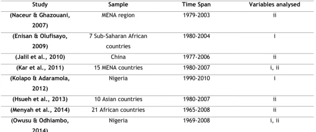
The supply-leading hypothesis contends unidirectional causality between variables. In this hypothesis, we either have causality running from stock market development to economic growth or we have causality running from banking sector development to economic growth. In the table below it is shown a summary of the studies confirming the supply-leading hypothesis.

Table 2. Studies confirming the supply-leading hypothesis.

(Naceur & Ghazouani, 2007)

MENA region 1979-2003 ii

(Enisan & Olufisayo, 2009)

7 Sub-Saharan African countries

1980-2004 i

(Jalil et al., 2010) China 1977-2006 ii

(Kar et al., 2011) 15 MENA countries 1980-2007 i, ii

(Kolapo & Adaramola, 2012)

Nigeria 1990-2010 i

(Hsueh et al., 2013) 10 Asian countries 1980-2007 ii

(Menyah et al., 2014) 21 African countries 1965-2008 ii

(Owusu & Odhiambo, 2014)

Nigeria 1969-2008 i, ii

Note: Due to different variables analysed in different studies it was used two letters to specify the causal relationship in study; i: study analyses the relationship between stock market development and economic growth; ii: study analyses the relationship between banking sector development and economic growth.

(23)

4

2.3. Demand-following hypothesis

Just like the supply-leading hypothesis, the demand-following hypothesis contends unidirectional causality between variables but in contrast, in the demand-following hypothesis the causality runs from economic growth to either stock market development or banking sector development. In the table below it is shown a summary of the studies confirming the demand-following hypothesis.

Table 3. Studies confirming the demand-following hypothesis

(Liu & Sinclair, 2008) China 1973-2003 i

(Ang, 2008) Malaysia 1960-2001 i

(Panopoulou, 2009) 5 countries 1995-2007 i, ii

(Kar et al., 2011) 15 MENA countries 1980-2007 i, ii

(Pradhan et al., 2014) 15 Asian countries 2011 i

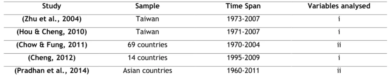
2.4. Feedback hypothesis

The existence of bidirectional causality between variables is known as the feedback hypothesis whereby the causality runs in both directions. In the table below is shown some studies confirming the feedback hypothesis.

Table 4. Studies confirming the feedback hypothesis

(Zhu et al., 2004) Taiwan 1973-2007 i

(Hou & Cheng, 2010) Taiwan 1971-2007 i

(Chow & Fung, 2011) 69 countries 1970-2004 ii

(Cheng, 2012) 14 countries 1995-2009 i

(Pradhan et al., 2014) Asian countries 1960-2011 ii

(24)

5

3. Data and methodology

This section refers to the data and the methodology applied. The data is described in section 3.1. in which it is possible to see the variables description in Table 5 as well as the sources and the definition of each variable. The methodology applied is explained in section 3.2.

3.1. Data

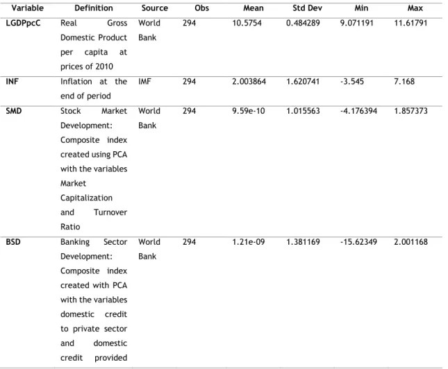
This paper uses annual data from 2001 to 2014 applied to a panel of 21 high income countries classified by the World Bank. The countries are Australia, Austria, Belgium, Greece, France, Germany, Ireland, Israel, Italy, Japan, Netherlands, Norway, Portugal, Singapore, Spain, USA, Poland, Switzerland, Slovenia, China (Hong Kong SAR) and Luxembourg. The variables of this study are real Gross Domestic Product per capita, inflation, stock market development and banking sector development. To create single variables that allow the assessment of stock market development and banking sector development, was used principal component analysis (PCA). To create stock market development, was used market capitalization of listed domestic companies and turnover ratio. Regarding banking sector development, was used domestic credit to private sector and domestic credit provided by the financial sector. The time horizon and the countries were chosen due to data availability for high income countries. The table below shows the variables, the definitions of them, source and summary statistics.

Table 5. Variables description.

Variable Definition Source Obs Mean Std Dev Min Max

LGDPpcC Real Gross Domestic Product per capita at prices of 2010 World Bank 294 10.5754 0.484289 9.071191 11.61791

INF Inflation at the

end of period

IMF 294 2.003864 1.620741 -3.545 7.168

SMD Stock Market

Development: Composite index created using PCA with the variables Market Capitalization and Turnover Ratio World Bank 294 9.59e-10 1.015563 -4.176394 1.857373 BSD Banking Sector Development: Composite index created with PCA with the variables domestic credit to private sector and domestic credit provided World Bank 294 1.21e-09 1.381169 -15.62349 2.001168

(25)

6

by the financial sector

Note: The letter L before variables denote natural logarithms; all monetary variables are in US dollars

To measure economic growth was used Real Gross Domestic product per capita at prices of 2010 in natural logarithms and the data was collected from the World Bank. To measure inflation, it was used inflation at the end of the period and the data was obtained from the IMF (International Monetary Fund) database. The variables Stock Market Development and Banking Sector Development were created using PCA. The PCA transforms original sets of variables into smaller sets of linear combinations that account for most of the variance of the original set. In other words, the use of this technique allows removing the essential information from each variable and it turns into a single composite variable that contains information from the various variables. In this case, Market Capitalization of listed domestic companies (divided by GDP) and Turnover ratio were the variables chosen to perform PCA to create Stock Market Development. It was used the test of Kaiser-Meyer-Olkin of sampling adequacy (Kaiser, 1970) and Bartlett’s test for sphericity (Bartlett, 1950) to test the robustness of the variable Stock Market Development (SMD) and the variable Banking Sector Development (BSD). The results for this test for the variable Stock Market Development is shown in the Table 6.

Table 6. Bartlett test of sphericity and Kaiser-Meyer-Olkin Measure of Sampling Adequacy for

the construction of SMD

Bartlett test of sphericity

Chi-square 0.287

Degree of freedom 1

p-value 0.592

Determinant of the correlation matrix 0.999

Kaiser-Meyer-Olkin Measure of Sampling Adequacy 0.500

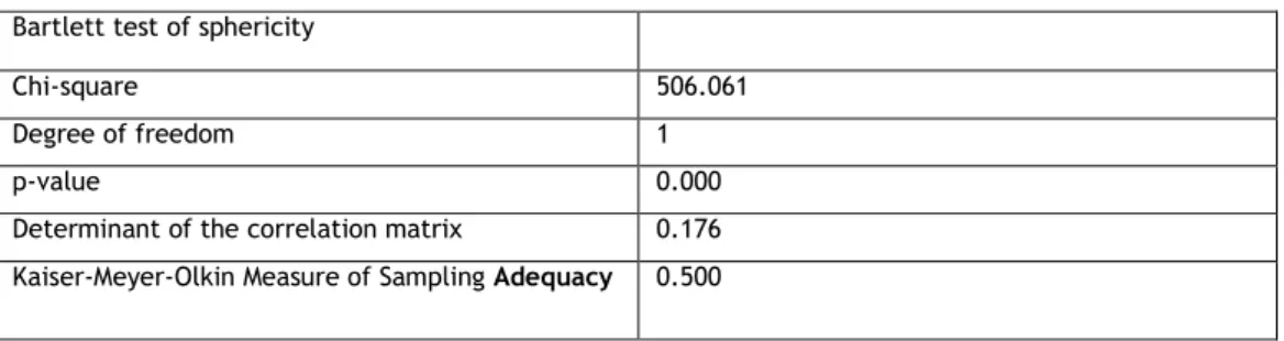
Regarding Banking Sector Development, was used domestic credit to private sector (% GDP) and domestic credit provided by the financial sector (% GDP). The results of the tests to the variable Banking Sector Development are shown in Table 7. All data was obtained from the World Bank.

Table 7. Bartlett test of sphericity and Kaiser-Meyer-Olkin Measure of Sampling Adequacy for

the construction of BSD

Bartlett test of sphericity

Chi-square 506.061

Degree of freedom 1

p-value 0.000

Determinant of the correlation matrix 0.176

Kaiser-Meyer-Olkin Measure of Sampling Adequacy 0.500

(26)

7 The null hypothesis for the Bartlett test of sphericity is that variables are not intercorrelated and in the case of BSD the null hypothesis was not rejected.

When the determinant of the correlation matrix is less than 1, all correlations are different than 0. If all correlations are equal to 0 the value of the determinant of the correlation matrix would be 1 but in this case, the test came up with a value of 0.962 meaning that all correlations are different than 0.

The Kaiser-Meyer-Olkin Measure of Sampling Adequacy takes a value between 0 and 1 and if it comes out below 0.5 the PCA should not be applied. In this case the Kaiser-Meyer-Olkin Measure of Sampling Adequacy is 0.5 for both variables meaning the PCA is possible to use.

3.2. Methodology

The methodology used in this dissertation was the same developed by Love & Zicchino (2006) in which is applied a panel-data vector autoregressive (PVAR) model. This technique combines the traditional VAR approach, which treats all the variables in the system as endogenous, with the panel-data approach allowing for unobserved individual heterogeneity (Grossmann et al., 2014). The equation for this model which is a first-order PVAR is specified as follows in eq. 1:

𝑧𝑖𝑡= Γ0+ Γ1𝑧𝑖𝑡−1+ 𝑓𝑖+ 𝑑𝑐,𝑡+ 𝑒𝑡 (1)

In this equation, 𝑧𝑡 is a four-variable vector {DLGDPpcC, DINF, DSMD, DBSD} in which all the

variables are stationary and in their first differences. This equation designates also the matrix polynomial, the fixed effects in the model, the time effects and the random errors term. Since the fixed effects are correlated with the regressors due to lags of the dependent variables, the mean-differencing procedure commonly used to eliminate fixed effects would create biased coefficients. To avoid this problem Love & Zicchino (2006) applied a technique called the ‘Helmert procedure’ (Arellano & Bover, 1995) which will also be applied in this dissertation’s model.

It was used the Generalized Method of Moments (GMM) estimator; the Granger causality test to analyse the causal relationship between the variables; the variance decomposition that shows the percent of the variation in one variable that is explained by the shock to another variable that accumulate over time showing the magnitude of the total effect and like Love & Zicchino (2006), the variance decomposition was analysed for 10 years; the impulse-response functions were computed and to analyse them, an estimate of their confidence intervals is needed. Since the matrix of impulse-response functions is constructed from the estimated VAR coefficients, their standard errors need to be taken into consideration. These standard errors of the impulse-response functions are calculated and confidence intervals are generated with Monte Carlo simulations.

(27)

8

4. Preliminary tests

To test the properties of the variables, several preliminary tests were performed. This section shows tests for heteroskedasticity, multicollinearity throughout the Variance Inflation Test (VIF), fixed/random effects throughout the Hausman test and cross section dependence throughout the Pesaran CD test (Pesaran, 2004). The results of these tests can be seen in the following tables.

Table 8. VIF test

Variable VIF 1/VIF Variable VIF 1/VIF

BSD 1.05 0.950145 DBSD 1.00 0.997954

INF 1.05 0.952813 DINF 1.00 0.997761

SMD 1.01 0.992148 DSMD 1.00 0.998626

Mean VIF 1.04 Mean VIF 1.00

As it can be seen in Table 8, the values of mean VIF for the variables and at first differences are, respectively, 1.04 and 1.00. Since they take a value below 10, there is no multicollinearity problems between the variables.

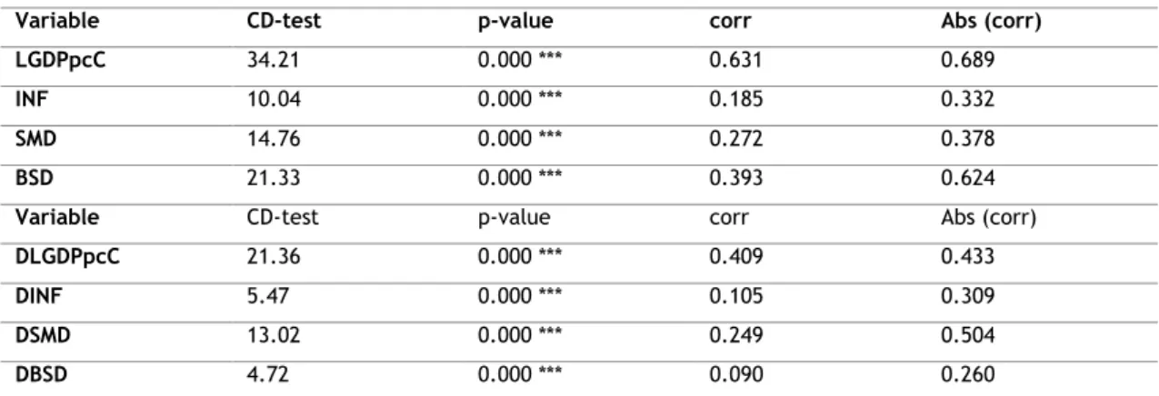
Table 9. Pesaran CD-test

Variable CD-test p-value corr Abs (corr)

LGDPpcC 34.21 0.000 *** 0.631 0.689

INF 10.04 0.000 *** 0.185 0.332

SMD 14.76 0.000 *** 0.272 0.378

BSD 21.33 0.000 *** 0.393 0.624

Variable CD-test p-value corr Abs (corr)

DLGDPpcC 21.36 0.000 *** 0.409 0.433

DINF 5.47 0.000 *** 0.105 0.309

DSMD 13.02 0.000 *** 0.249 0.504

DBSD 4.72 0.000 *** 0.090 0.260

Note: *** denotes 1% statistical significance; Stata command xtcd was used.

In Table 9, are demonstrated the results for the Average correlation coefficients & Pesaran (2004) CD test. The null hypothesis of this test is cross-section independence CD ~N(0,1) and in this case we can see the presence of cross-section dependence in levels and at first differences and because of this, the procedure is to execute the 2nd_{generation of unit root test. However,} because the time span is very little the 2nd_{generation of unit root test is not much relevant for} the study so the results were not displayed.

(28)

9

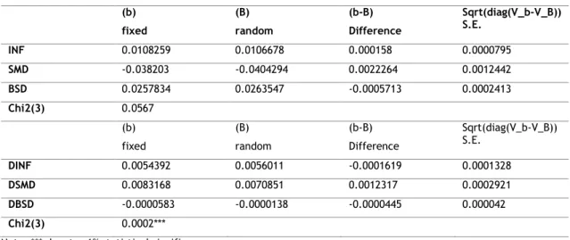
Table 10. Hausman test

(b) fixed (B) random (b-B) Difference Sqrt(diag(V_b-V_B)) S.E. INF 0.0108259 0.0106678 0.000158 0.0000795 SMD -0.038203 -0.0404294 0.0022264 0.0012442 BSD 0.0257834 0.0263547 -0.0005713 0.0002413 Chi2(3) 0.0567 (b) fixed (B) random (b-B) Difference Sqrt(diag(V_b-V_B)) S.E. DINF 0.0054392 0.0056011 -0.0001619 0.0001328 DSMD 0.0083168 0.0070851 0.0012317 0.0002921 DBSD -0.0000583 -0.0000138 -0.0000445 0.000042 Chi2(3) 0.0002***

Note: *** denotes 1% statistical significance.

In Table 10 are demonstrated the results for the Hausman test which null hypothesis is difference in coefficients are not systematic. In the case of our model we have a fixed effects model (p-value = 0.0002, which is <0.05) for the variables in their first differences and a random effect model for the variables. Because we must work with a fixed effect model, we will use the variables in their first differences.

Table 11. Lag order selection

Lag CD J J p-value MBIC MAIC MQIC

1 0.9939296 81.30077 0.0018988 -164.6495 -14.69923 -75.55635

2 0.9883348 54.57506 0.0076978 -109.3918 -9.424937 -49.99635

3 0.9955902 31.25528 0.0124809 -50.72815 -0.7447225 -21.03043

4 0.9362655 . . . . .

Note: Stata command pvarsoc was used.

In Table 11 we have the results for the lag order selection. This step is mentioned in the methodology section as it is followed Grossmann et al. (2014) procedure which calculates the overall coefficient of determination (CD), Hansen’s J statistic (J), J p-value and the three model selection criteria by Andrews & Lu (2001) which are MBIC, MAIC and MQIC. It was used a maximum of 4 lags totalizing 168 observations, 21 panels and an Average number of T of 8. Since the MBIC and MQIC values are lower at one lag, it was selected a first-order PVAR.

(29)

10

5. Empirical results

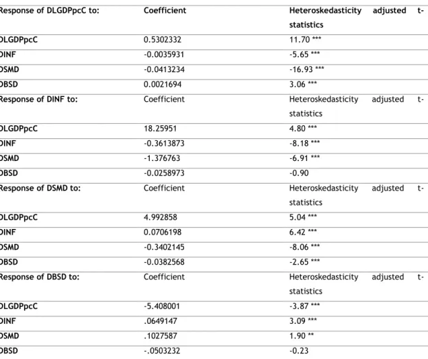
This section shows the empirical results of this paper. A PVAR was estimated using one lag and all variables are in their first differences. The option gmmst (in the pvar command) was used replacing missing values with zero (Holtz-Eakin et al., 1988). This procedure enlarges the number of observations resulting in more efficient results. Table 12 shows the results for the VAR model estimated.

Table 12. VAR model results

Response of DLGDPpcC to: Coefficient Heteroskedasticity adjusted

t-statistics

DLGDPpcC 0.5302332 11.70 ***

DINF -0.0035931 -5.65 ***

DSMD -0.0413234 -16.93 ***

DBSD 0.0021694 3.06 ***

Response of DINF to: Coefficient Heteroskedasticity adjusted

t-statistics

DLGDPpcC 18.25951 4.80 ***

DINF -0.3613873 -8.18 ***

DSMD -1.376763 -6.91 ***

DBSD -0.0258973 -0.90

Response of DSMD to: Coefficient Heteroskedasticity adjusted

t-statistics

DLGDPpcC 4.992858 5.04 ***

DINF 0.0706198 6.42 ***

DSMD -0.3402145 -8.06 ***

DBSD -0.0382568 -2.65 ***

Response of DBSD to: Coefficient Heteroskedasticity adjusted

t-statistics

DLGDPpcC -5.408001 -3.87 ***

DINF .0649147 3.09 ***

DSMD .1027587 1.90 **

DBSD -.0503232 -0.23

Note: *** and ** denote statistical significance level of, respectively, 1% and 5%. The Stata command pvar with the option gmmst with one lag was used.

(30)

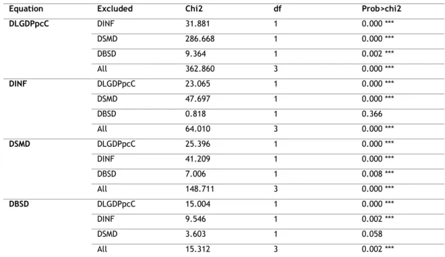
11 The Wald test was used to evaluate the Granger causality. The Table 13 shows the results for the PVAR Granger causality Wald test and we can see there is bidirectional causality between real GDP per capita constant and Inflation as well as between GDP per capita constant and Stock Market Development, GDP per capita constant and Banking Sector Development and between inflation and Stock Market Development. We can also see unidirectional causality between Inflation and Banking Sector Development as well as between Stock Market Development and Banking Sector Development.

Table 13. Granger causality test

Equation Excluded Chi2 df Prob>chi2

DLGDPpcC DINF 31.881 1 0.000 *** DSMD 286.668 1 0.000 *** DBSD 9.364 1 0.002 *** All 362.860 3 0.000 *** DINF DLGDPpcC 23.065 1 0.000 *** DSMD 47.697 1 0.000 *** DBSD 0.818 1 0.366 All 64.010 3 0.000 *** DSMD DLGDPpcC 25.396 1 0.000 *** DINF 41.209 1 0.000 *** DBSD 7.006 1 0.008 *** All 148.711 3 0.000 *** DBSD DLGDPpcC 15.004 1 0.000 *** DINF 9.546 1 0.002 *** DSMD 3.603 1 0.058 All 15.312 3 0.002 ***

(31)

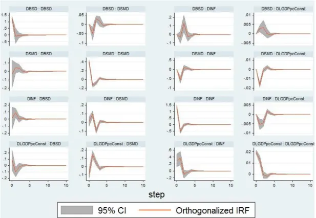
12 In Figure 1, which is displayed above, we can observe the impulse-response functions where all variables return to zero after a shock in a maximum of five years meaning that all variables are stationary, what comes in line with the previous results in the preliminary tests. This system is a reactive system that after a few periods all variables return to the equilibrium by a harmonic movement. We can observe an expected positive reaction of DLGDPpcC in response to both DSMD and DBSD, coming in line with the literature.

Figure 1. Impulse-response functions

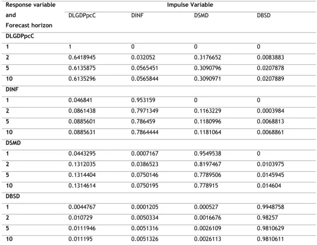
In Table 14 we have the results for the forecast-error variance decomposition, which represents how a variable respond to shocks in specific variables (Marques, Fuinhas, & Marques, 2013). These results are consistent with the results from the Hausman test and the impulse-response functions. Regarding DLGDPpcC, after a 2-year period, shocks to DLGDPpcC explain about 64% of the forecast error variance and after 10 years it stabilizes at 61%. The shocks to DINF explain about 5.6% while the shocks to DSMD and DBSD explain, respectively, 30.9% and 2.07%. Considering DINF in year period, shocks to DINF explain 95.3% of the forecast error variance and after a 10-year period this percentage changes to 78.6% while DLGDPpcC explains 8.86%, DSMD explains 11.8% and DBSD explains 0.69%. Analysing the impacts on DSMD, a shock on DSMD explain 95.5% of the forecast error variance decomposition after one year and 77.89% after 10 years. DLGDPpcC explains 13.1%, DINF explains 7.5% and DBSD explains 1.46%. Regarding the impacts on DBSD, a shock after one year on DBSD explains 99.49% and 98.1% after 10 years. In

(32)

13 this model the variable DBSD is the most autonomous being almost autoregressive because it auto explains 98.1% after 10 years and the remaining variables have a very low impact on DBSD.

Table 14. Forecast-error variance decomposition

Response variable and Forecast horizon Impulse Variable DLGDPpcC DINF DSMD DBSD DLGDPpcC 1 1 0 0 0 2 0.6418945 0.032052 0.3176652 0.0083883 5 0.6135875 0.0565451 0.3090796 0.0207878 10 0.6135296 0.0565844 0.3090971 0.0207889 DINF 1 0.046841 0.953159 0 0 2 0.0861438 0.7971349 0.1163229 0.0003984 5 0.0885601 0.786459 0.1180996 0.0068813 10 0.0885631 0.7864444 0.1181064 0.0068861 DSMD 1 0.0443295 0.0007167 0.9549538 0 2 0.1312035 0.0386523 0.8197467 0.0103975 5 0.1314404 0.0750146 0.7789506 0.0145945 10 0.1314614 0.0750195 0.778915 0.014604 DBSD 1 0.0044767 0.0001205 0.000527 0.9948758 2 0.010729 0.0050334 0.0016676 0.98257 5 0.0111946 0.0051316 0.0026109 0.9810629 10 0.011195 0.0051326 0.0026113 0.9810611

Note: Stata command pvarfevd was used.

To check the robust of the PVAR was performed a stability test. This tests the condition of eigenvalues. The Figure 2 shows the results in which all eigenvalues are inside the circle unit meaning PVAR satisfies stability condition (Hamilton, 1994; Lutkephol, 2005).

Figure 2. Eigenvalue stability condition

Note: Stata command pvarstable was used.

Eigenvalue

Real Imaginary Modulus

0.0041056 -0.3263796 0.3264054

0.0041056 0.3263796 0.3264054

-0.1149515 0.1679139 0.2034918

(33)

14

6. Conclusion

This paper applies a PVAR model, Granger causality test, impulse-response functions and forecast-error variance decomposition to study the causal nexus between economic growth, inflation, stock market development and banking sector development for 21 countries from 2001 to 2014. The variables Stock Market Development and Banking Sector Development were created using PCA method. This method proved to be very useful because throughout it, the assessment of these 2 sub-categories of the financial development was easier instead of working with more variables. Market capitalization of listed domestic companies and turnover ratio were the variables chosen to perform PCA to create Stock Market Development (SMD) meanwhile domestic credit to private sector and domestic credit provided by the financial sector were the variables chosen to perform PCA to create Banking Sector Development (BSD). It was also used real gross domestic product per capita constant as a proxy of economic growth and a macroeconomic variable such as inflation at the end of period.

In the literature review, four theories regarding the causality between variables were highlighted: the null hypothesis (no causality between variables), supply-leading and demand-following hypotheses (unidirectional causality between variables) and feedback hypothesis (bidirectional causality between variables). As we could conclude from above, we have found bidirectional causality between real GDP per capita constant and Inflation as well as between real GDP per capita constant and Stock Market Development, real GDP per capita constant and Banking Sector Development and between inflation and Stock Market Development. This confirms the feedback theory. We also found the existence of unidirectional causality between Inflation and Banking Sector Development as well as between Stock Market Development and Banking Sector Development. This follows the supply-leading theory.

Through the impulse-response functions we can conclude that all variables return to zero after a shock in a maximum of five years. We can also see a positive impact on economic growth in response to banking sector development and stock market development, coming in line with the literature that a well-developed financial system is growth-enhancing following the proposition of “more finance, more growth”.

(34)

15

Referências

Andrews, D. K., & Lu, B. (2001). Consistent model and moment selection procedures for GMM estimation with application to dynamic panel data models. Journal of Econometrics,

101(1), 123-164.

Ang, J. B. (2008). Survey of recent developments in the literature of finance and growth.

Journal of Economic Surveys, 22(3), 536-576.

Arellano, M., & Bover, O. (1995). Another look at the instrumental variable estimation of error components models. Journal of Econometrics, 68, 29-51.

Beck, T., & Levine, R. (2004). Stock Markets, banks, and growth: Panel evidence. Journal of

Banking and Finance, 28(3), 423-442.

Bencivenga, V., & Smith, B. (1991). Financial intermediation and endogenous growth. Review

of Economic Studies, 195-209.

Bencivenga, V., Smith, D. B., & Starr, M. R. (1995). Transaction costs, technological choice, endogenous growth. Journal of Economic Theory, 67(1), 53-117.

Cheng, S. (2012). Substitution or complementary effects between banking and stock markets: evidence from financial openness. Journal of International Financial Markets,

Institutions and Money, 22(3), 508-520.

Chow, W. W., & Fung, M. K. (2011). Financial development and growth: A clustering and causality analysis. Journal of International Trade and Economic Development, 35(3), 1-24.

Enisan, A., & Olufisayo, O. (2009). Stock Market Development and Economic Growth: Evidence from seven sub-Sahara African countries. Journal of Economics and Business 61(2), 162-171.

Fink, G., Haiss, P., & Vuksic, G. (2009). Contribution of financial market segments at different stages of development: Transition, cohesion and mature economies compared. Journal

of Financial Stability, 5(4), 431-455.

Fung, K. M. (2009). Financial development and economic growth: Convergence or divergence?

Journal of International Money and Finance, 28(1), 56-67.

Garcia, F. V., & Liu, L. (1999). Macroeconomic determinants of stock market development .

Journal of Applied Economics, 11(1), 29-59.

Greenwood, J., & Jovanovic, B. (1990). Financial development, growth, and the distribution of income. Journal of Political Economy, 1076-1107.

(35)

16 Grossmann, A., Love, I., & Orlov, A. (2014). The dynamics of exchange rate volatility: A panel VAR approach. Journal of International Financial Markets, Institutions and Money, 1-27.

Hamilton, J. (1994). Time series analysis. Prentice Hall New Jersey 1994, SFB 373(Chapter 5), 837-900.

Holtz-Eakin, D., Newey, W., & Rosen, H. (1988). Estimating Vector Autoregressions with Panel Data. Econometrica, 1371-1395.

Hou, H., & Cheng, Y. (2010). The roles of stock market in the finance-growth nexus: time series cointegration and causality evidence from Taiwan. Applied Financial Economics,

20(12), 975-981.

Hsueh, S., Hu, Y., & Tu, C. (2013). Economic growth and financial development in Asian countries: A bootstrap panel Granger causality analysis. Economic Modelling, 32(3), 295-301.

Jalil, A., Feridun, M., & Ma, Y. (2010). Finance-growth nexus in China revisited: New evidence from principal components and ARDL bounds tests. International Review of Economics

and Finance, 19(2), 189-195.

Kar, M., Nazlioglu, S., & Agir, H. (2011). Financial development and economic growth nexus in the MENA countries: Bootstrap panel granger causality analysis. Economic Modelling, 685-693.

Kolapo, T., & Adaramola, O. (2012). The impact of the Nigerian Capital Market on Economic Growth (1990-2010). International Journal of Developing Societies, 11-19.

Law, S., & Singh, N. (2014). Does too much finance harm economic growth? Journal of Banking

and Finance, 36-44.

Levine, R., & Zervos, S. (1998). Stock markets, banks and economic growth. American Economic

Review, 88(3), 537-558.

Liu, X., & Sinclair, P. (2008). Does the linkage between stock market performance and economic growth vary across Greater China? Applied Economics Letters, 15, 505-508.

Love, I., & Zicchino, L. (2006). Financial development and dynamic investment behaviour: evidence from panel VAR. The Quarterly Review of Economics and Finance, 46(2), 190-210.

Lutkephol, H. (2005). New Introduction to Multiple Time Series Analysis.

Marques, L. M., Fuinhas, J. A., & Marques, A. C. (2013). Does the stock market causa economic growth? Portuguese evidence of economic regime change. Economic Modelling, 32, 316-324.

(36)

17 Menyah, K., Nazlioglu, S., & Wolde-Rufael, Y. (2014). Financial development, trade openess and economic growth in African countries: New insights from a panel causality approach. Economic Modelling, 37(2), 386-394.

Naceur, B. S., & Ghazouani, S. (2007). Stock markets, banks and economic growth: Empirical evidence from the MENA region. Research in International Business and Finance, 21(2), 297-315.

Owusu, L. E., & Odhiambo, M. N. (2014). Financial liberalization and economic growth in Nigeria: An ARDL-bounds testing approach. Journal of Economic Policy Reform, 17(2), 164-177.

Panopoulou, E. (2009). Financial variables and euro area growth: A non-parametric causality analysis. Economic Modelling 26(6), 1414-1419.

Pesaran, M. (2004). General diagnostics tests for cross section dependence in panels. Iza, 1-42. Pradhan, R. P., Arvin, M. B., Norman, N. R., & Nishigaki, Y. (2014). Does banking sector development affect economic growth and inflation? A panel cointegration and causality approach. Applied Financial Economics, 24(7), 465-480.

Pradhan, R., Arvin, M., Bahmani, S., Hall, J., & Norman, N. (2017). Finance and growth: Evidence from the ARF countries. The Quarterly Review of Economics and Finance. Pradhan, R., Arvin, M., Samadhan, B., & Taneja, S. (2013). The Impact of Stock Market

Development on inflation and Economic Growth of 16 Asian Countries: A Panel VAR Approach. Applied Econometrics and International Development Vol.13-1.

Rousseau, L. P., & Xiao, S. (2007). Equity Markets and Growth: Cross Country Evidence on Timing and Outcomes. Journal of Banking and Finance, 24(12), 1933-1957.

Schumpeter. (1911). The Theory of Economic Development. Cambridge: Harvard University Press.

Zhu, A., Ash, M., & Pollin, R. (2004). Stock market liquidity and economic growth: a critical appraisal of the Levine/Zervos model. International Review of Applied Economics,