DEPARTAMENTO DE INFORMÁTICA
BICLUSTERING ELECTRONIC HEALTH RECORDS TO
UNRAVEL DISEASE PRESENTATION PATTERNS
Joana Sofia Santos de Matos
Mestrado em Ciência de Dados
Dissertação orientada por:
“There are only patterns, patterns on top of patterns, patterns that affect other patterns. Patterns hidden by patterns. Patterns within patterns.
If you watch close, history does nothing but repeat itself. What we call chaos is just patterns we haven’t recognized.”
This work would not have been possible without the FCT funding to NEUROCLINOMICS2 (PTDC/EEI-SII/1937/2014) research project, and the LASIGE Research Unit’s (UID/CEC/00408/2019) hosting.
First of all, I would like to thank the team involved in the project, from Faculdade de Ciências da Universidade de Lisboa (FCUL) and Instituto de Medicina Molecular (IMM) João Lobo Antunes: my advisor, Prof. Sara Madeira, for her guidance and support; Dr. Mamede de Carvalho for his indispensable knowledge and experience; Manuel Figueiredo and Marta Gromicho for validating and correcting the data; and Sofia Pires for her help in creating the class labelling used in the second Task. Additionally, I would also like to thank Rui Henriques from Instituto Superior Técnico (IST) for his aid in how to use the BicPAMS algorithm for our experiments.
In the past year, I had the privilege of meeting many awesome people here at LASIGE, whom I already consider my friends. I’ll dearly miss the companionship we built during our meal times and festive events, so I really hope we won’t lose contact!
Last but not least, I want to thank my family. Most of all my parents, Albano and Maria João, for their loving encouragement of my tardy pursuit of a master’s degree, and my dear husband-to-be, Pedro, for his endless patience and love during this endeavor.
A Esclerose Lateral Amiotrófica (ELA) é uma doença neurodegenerativa heterogénea com padrões de apresentação altamente variáveis. Dada a natureza heterogénea dos doentes com ELA, aquando do di-agnóstico os clínicos normalmente estimam a progressão da doença utilizando uma taxa de decaimento funcional, calculada com base na Escala Revista de Avaliação Funcional de ELA (ALSFRS-R).
A utilização de modelos de Aprendizagem Automática que consigam lidar com este padrões com-plexos é necessária para compreender a doença, melhorar os cuidados aos doentes e a sua sobrevivência. Estes modelos devem ser explicáveis para que os clínicos possam tomar decisões informadas.
Desta forma, o nosso objectivo é descobrir padrões de apresentação da doença, para isso propondo uma nova abordagem de Prospecção de Dados: Descoberta de Meta-atributos Discriminativos (DMD), que utiliza uma combinação de Biclustering, Classificação baseada em Biclustering e Prospecção de Re-gras de Associação para Classificação. Estes padrões (chamados de Meta-atributos) são compostos por subconjuntos de atributos discriminativos conjuntamente com os seus valores, permitindo assim distin-guir e caracterizar subgrupos de doentes com padrões similares de apresentação da doença.
Os Registos de Saúde Electrónicos (RSE) utilizados neste trabalho provêm do conjunto de dados JPND ONWebDUALS (ONTology-based Web Database for Understanding Amyotrophic Lateral
Scle-rosis), composto por questões standardizadas acerca de factores de risco, mutações genéticas, atributos
clínicos ou informação de sobrevivência de uma coorte de doentes e controlos seguidos pelo consórcio ENCALS (European Network to Cure ALS), que inclui vários países europeus, incluindo Portugal.
Nesta tese a metodologia proposta foi utilizada na parte portuguesa do conjunto de dados ONWebD-UALS para encontrar padrões de apresentação da doença que: 1) distinguissem os doentes de ELA dos seus controlos e 2) caracterizassem grupos de doentes de ELA com diferentes taxas de progressão (cat-egorizados em grupos Lentos, Neutros e Rápidos). Nenhum padrão coerente emergiu das experiências efectuadas para a primeira tarefa. Contudo, para a segunda tarefa os padrões encontrados para cada um dos três grupos de progressão foram reconhecidos e validados por clínicos especialistas em ELA, como sendo características relevantes de doentes com progressão Lenta, Neutra e Rápida. Estes resultados sug-erem que a nossa abordagem genérica baseada em Biclustering tem potencial para identificar padrões de apresentação noutros problemas ou doenças semelhantes.
Palavras Chave: Esclerose Lateral Amiotrófica, Biclustering baseado em Prospecção de Padrões,
Classificação baseada em Biclustering, Prospecção de Regras de Associação para Classificação,
Amyotrophic Lateral Sclerosis (ALS) is a heterogeneous neurodegenerative disease with a high vari-ability of presentation patterns. Given the heterogeneous nature of ALS patients and targeting a better prognosis, clinicians usually estimate disease progression at diagnosis using the rate of decay computed from the Revised ALS Functional Rating Scale (ALSFRS-R).
In this context, the use of Machine Learning models able to unravel the complexity of disease pre-sentation patterns is paramount for disease understanding, targeting improved patient care and longer survival times. Furthermore, explainable models are vital, since clinicians must be able to understand the reasoning behind a given model’s result before making a decision that can impact a patient’s life.
Therefore we aim at unravelling disease presentation patterns by proposing a new Data Mining ap-proach called Discriminative Meta-features Discovery (DMD), which uses a combination of Bicluster-ing, Biclustering-based Classification and Class Association Rule Mining. These patterns (called Meta-features) are composed of discriminative subsets of features together with their values, allowing to dis-tinguish and characterize subgroups of patients with similar disease presentation patterns.
The Electronic Health Record (EHR) data used in this work comes from the JPND ONWebDUALS (ONTology-based Web Database for Understanding Amyotrophic Lateral Sclerosis) dataset, comprised of standardized questionnaire answers regarding risk factors, genetic mutations, clinical features and survival information from a cohort of patients and controls from ENCALS (European Network to Cure ALS), a consortium of diverse European countries, including Portugal.
In this work the proposed methodology was used on the ONWebDUALS Portuguese EHR data to find disease presentation patterns that: 1) distinguish the ALS patients from their controls and 2) characterize groups of ALS patients with different progression rates (categorized into Slow, Neutral and Fast groups). No clear pattern emerged from the experiments performed for the first task. However, in the second task the patterns found for each of the three progression groups were recognized and validated by ALS expert clinicians, as being relevant characteristics of slow, neutral and fast progressing patients. These results suggest that our generic Biclustering approach is a promising way to unravel disease presentation patterns and could be applied to similar problems and other diseases.
Keywords: Amyotrophic Lateral Sclerosis, Pattern Mining-based Biclustering, Biclustering-based
A Esclerose Lateral Amiotrófica (ELA) é uma doença neurodegenerativa heterogénea que afecta o Sis-tema Motor humano, num período de tempo relativamente curto. A doença pode surgir numa determi-nada região do corpo e com o tempo afectar também outras. Alguns sintomas comuns são: fraqueza nos membros, dificuldades em falar e engolir, insuficiência respiratória e alterações cognitivas/compor-tamentais. A principal causa de morte é a eventual insuficiência respiratória. O tempo de sobrevivência é altamente variável, dependendo da velocidade da progressão da doença, que aquando do diagnóstico é frequentemente estimada pelos clínicos utilizando uma taxa de decaimento funcional, calculada com base na Escala Revista de Avaliação Funcional de ELA (ALSFRS-R). Esta escala é composta por 12 perguntas cujo valor para cada uma varia entre 0 e 4, com um valor máximo de 48 (quanto maior o valor total, maior a capacidade funcional do doente).
Até ao presente dia, continua a ser necessário descobrir testes de diagnóstico fiáveis ou biomarcadores que ajudem os clínicos a conseguir diagnosticar esta doença de forma rápida e eficaz, dado o alto grau de variabilidade existente nos fenótipos observados, história familiar, genes envolvidos, vias moleculares e factores ambientais que a poderão provocar. Tendo isto em consideração, acredita-se que existem diversos mecanismos que podem causar a neurodegenerescência em doentes com ELA.
Dentro deste contexto, o nosso objectivo é descobrir padrões de apresentação da doença. Estes padrões (que neste trabalho serão chamados de Meta-atributos) são compostos por subconjuntos de atrib-utos discriminativos conjuntamente com os seus valores, permitindo assim distinguir e caracterizar sub-grupos de doentes com padrões similares de apresentação da doença. Uma possível forma de identificar este tipo de padrões é através da utilização de modelos de Aprendizagem Automática, que conseguem li-dar com a complexidade dos mesmos, permitindo compreender melhor a doença, criar tratamentos mais específicos para os doentes e aumentar o seu tempo de sobrevivência. Idealmente, esses modelos dev-erão ser explicáveis, uma vez que os clínicos têm de conseguir compreender o raciocínio por detrás de um resultado do modelo antes de tomar qualquer decisão com impacto na vida de um doente.
Os Registos de Saúde Electrónicos (RSE) utilizados neste trabalho provêm do conjunto de dados JPND ONWebDUALS (ONTology-based Web Database for Understanding Amyotrophic Lateral
Scle-rosis), composto por questões standardizadas acerca de factores de risco, mutações genéticas, atributos
clínicos ou informação de sobreviência de uma coorte de doentes e controlos seguidos pelo consórcio ENCALS (European Network to Cure ALS), que inclui vários países europeus, incluindo Portugal.
Assim, neste trabalho é proposta uma nova abordagem exploratória para a Prospecção de Dados, chamada Descoberta de Meta-atributos Discriminativos (DMD). A base da mesma assenta na utilização
de dados bidimensionais. Até à data estas técnicas foram aplicadas com sucesso em dados médicos, per-mitindo descobrir grupos de entidades biológicas significativamente correlacionadas num subconjunto de condições ou pontos no tempo. De forma a encontrar Biclusters com sobreposição de forma eficiente utilizou-se uma variante - Biclustering baseado em Prospecção de Padrões - que necessita da prévia cat-egorização dos dados, o que pode implicar alguma perda de informação. Os Biclusters são considerados discriminativos caso pelo menos 75% das observações incluídas nos mesmos pertençam a uma dada classe, embora esta não seja considerada quando os Biclusters estão a ser prospectados. Entre vários conjuntos de Biclusters obtidos em experiências diferentes, foram considerados melhores os que tinham maior número de Biclusters discriminativos.
Sobre esses resultados são utilizadas técnicas de Classificação baseada em Biclustering e Prospecção de Regras de Associação para Classificação, para descobrir quais os padrões mais discriminativos para cada classe considerada. Por um lado a primeira abordagem utiliza uma matriz de identificadores dos sujeitos (doentes ou controlos) × identificadores dos Biclusters discriminativos que indica em que
Bi-clusters os sujeitos estavam presentes. Utilizando os identificadores dos BiBi-clusters como atributos,
con-seguimos verificar que conjuntos de atributos (e os seus valores) são considerados mais importantes na classificação e comparar com os atributos individuais. Por outro lado, a segunda abordagem tira partido da teoria de conjuntos para encontrar os subconjuntos de atributos (e os seus valores) que estão mais associados com cada classe. Estas duas abordagens foram utilizadas em paralelo para tirar partido das características explicativas dos modelos utilizados e também para validar a robustez dos resultados obti-dos. Várias experiências (incluindo baselines) foram incluídas para efeitos comparativos. Uma nota importante é a de que a abordagem DMD foi desenhada para ser genérica, podendo ser implementada de outras formas, utilizando outros algoritmos e até para tipos de dados diferentes, dependendo apenas das capacidades do algoritmo de Biclustering escolhido.
Nesta tese a implementação da metodologia DMD foi feita recorrendo a diversos softwares e lingua-gens de programação. O pré-processamento dos dados foi todo efectuado utilizando o software KNIME, incluindo a limpeza, transformação, categorização, adição de classe e selecção de atributos. O
Biclus-tering baseado em Prospecção de Padrões foi corrido utilizando o algoritmo BicPAM (que faz parte do software open-source BicPAMS), a partir de código Java criado para correr conjuntos de experiências
a partir de todas as combinações de parâmetros definidas (ExperienceSet). Adicionalmente foi criado código para traduzir os estágios intermédios dos Biclusters (de índices de categorias para valores de cat-egorias, e destes últimos para as etiquetas finais, mais legíveis), que ocorreram como consequência de trabalhar com dados categóricos no BicPAMS. A Classificação baseada em Biclustering foi feita uti-lizando a biblioteca scikit-learn para a linguagem Python, recorrendo a modelos Random Forest para obter métricas de importância dos atributos utilizados na classificação. Finalmente, a Prospecção de Regras de Associação para Classificação foi feita em Python, tirando partido da biblioteca open-source SPMF, escrita em Java.
Seguidamente, a metodologia proposta foi utilizada na parte portuguesa do conjunto de dados ON-WebDUALS para encontrar padrões de apresentação de ELA que: 1) distinguissem os doentes de ELA
algoritmo de Maximização de Expectativas).
Na primeira tarefa nenhum padrão coerente emergiu das experiências efectuadas, não tendo sido en-contrados resultados convergentes entre as técnicas de Classificação baseada em Biclustering e Prospecção de Regras de Associação para Classificação. Embora fosse uma tarefa mais complexa que a segunda, a selecção de atributos efectuada e o excesso de atributos vindos dos Biclusters discriminativos encontra-dos poderão ter contribuído para a ausência de resultaencontra-dos conclusivos. Contudo, foi possível verificar que não houve atributos individuais a serem apontados como os mais importantes para a classificação. Desta forma foi possível concluir que para distinguir os doentes dos controlos terão de ser considerados subconjuntos de atributos (e seus valores).
Na segunda tarefa foram encontrados padrões para cada um dos três grupos de progressão (Lenta, Neutra e Rápida), tendo sido reconhecidos e validados por clínicos especialistas em ELA. Os doentes de progressão Lenta foram identificados pelos valores consistentemente máximos de algumas pergun-tas da escala ALSFRS-R. Já para os doentes de progressão Neutra, a pergunta 5 da escala ALSFRS-R (relacionada com o corte de comida e manejar utensílios) com o valor 3, indicando algum decaimento funcional. Finalmente, os doentes de progressão rápida foram caracterizados pelos valores mais baixos dos atributos Atraso no diagnóstico e Tempo de transição entre a região 1 e 2.
Estes resultados sugerem que a nossa abordagem genérica baseada em Biclustering tem potencial para ser identificar padrões de apresentação noutros problemas ou doenças semelhantes.
1 Introduction 1
1.1 Context and Motivation . . . 1
1.2 ONWebDUALS dataset . . . 2
1.3 Objectives and Contributions . . . 3
1.4 Thesis Outline . . . 4
2 Background and Related Work 5 2.1 Amyotrophic Lateral Sclerosis . . . 5
2.2 Unsupervised Learning . . . 6
2.2.1 Clustering . . . 7
2.2.2 Biclustering . . . 7
2.2.3 Clustering vs Biclustering . . . 14
2.2.4 Pattern Mining . . . 14
2.2.5 Pattern-Mining based Biclustering . . . 16
2.3 Supervised Learning . . . 17
2.3.1 Classification . . . 17
2.3.2 Discriminative Biclustering . . . 26
2.3.3 Biclustering-Based Classification . . . 28
2.4 Association Rule Mining . . . 28
2.4.1 Rule Interest Metrics . . . 29
2.4.2 Filtering Uninteresting Association Rules . . . 29
2.4.3 Associative Classification . . . 30
2.5 Dimensionality Reduction . . . 30
2.5.1 Dimensionality Reduction for Categorical Data . . . 31
2.6 Related Work . . . 33
2.6.1 Biclustering in Healthcare Records . . . 33
2.6.2 Pattern Mining-Based Biclustering Algorithms . . . 33
2.6.3 Previous Uses of the ONWebDUALS data . . . 34
2.6.4 Progression Groups in ALS . . . 34
2.6.5 Biclustering-Based Classification in Healthcare . . . 35
3.1.1 Data Pre-processing . . . 38
3.1.2 Feature Selection . . . 41
3.1.3 Pattern Mining-based Biclustering . . . 42
3.1.4 Biclustering-based Classification . . . 46
3.1.5 Class Association Rule Mining . . . 46
3.1.6 Workflows and Code . . . 47
4 Discriminative Meta-features Discovery: A Case Study in the Portuguese ONWebDUALS Dataset 49 4.1 Task 1 - Discriminative Meta-features between Portuguese ALS Patients and Controls . . 49
4.1.1 Data and Settings . . . 49
4.1.2 Results and Discussion . . . 51
4.2 Task 2 - Discriminative Meta-features between Progression Groups on Portuguese ALS Patients . . . 62
4.2.1 Data and Settings . . . 62
4.2.2 Results and Discussion . . . 63
5 Conclusions and Future Work 75
References 77
Appendix A Discretized ONWebDUALS Dataset 85
Appendix B ONWebDUALS dataset features for Task 1 111
Appendix C ONWebDUALS dataset features for Task 2 115
1.1 Layout of the ONWebDUALS dataset. . . 2
2.1 Illustrative example of Clustering. . . 7
2.2 Illustrative example of a Biclustering solution. . . 8
2.3 Examples of different types of Biclusters (adapted from [44]). . . 9
2.4 Overlapping Biclusters with GAM (adapted from [44]). . . 11
2.5 Overlapping Biclusters with GMM (adapted from [44]). . . 11
2.6 Examples of different types of Bicluster structures (adapted from [44]). . . 12
2.7 Clustering and Biclustering Comparison (adapted from [18]). . . 14
2.8 Example of an itemset database D with the coverage and support of an itemset P . . . 15
2.9 Frequent, closed frequent and maximal frequent itemsets. . . 15
2.10 Illustrative example of a decision boundary on a Binary Classification problem. . . 18
2.11 Example of a Decision Tree built from the PlayTennis example dataset (adapted from [46]). 19 2.12 Receiver Operating Characteristic curve and Area Under Curve. . . 21
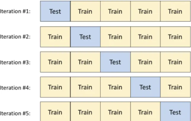
2.13 Division of an example dataset for each iteration in 5-fold Cross-Validation. . . 23
2.14 Inner workings of an Ensemble method (adapted from [22]). . . 24
2.15 Example of class-discriminative Biclusters’ mining. . . 27
2.16 Example of Subject × Biclusters Matrix for Biclustering-based Classification. . . 28
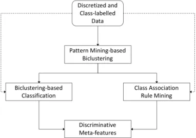
3.1 Simplified workflow of the proposed DMD approach. . . 38
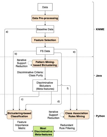
3.2 Detailed workflow of the proposed DMD approach. . . 39
3.3 Data Pre-processing steps and output. . . 39
3.4 Feature Selection steps and output. . . 42
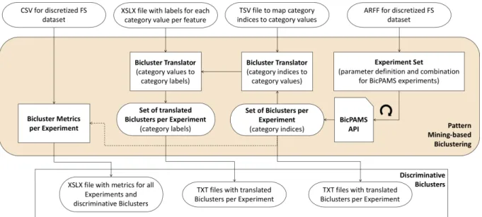
3.5 Pattern Mining-based Biclustering details. . . 42
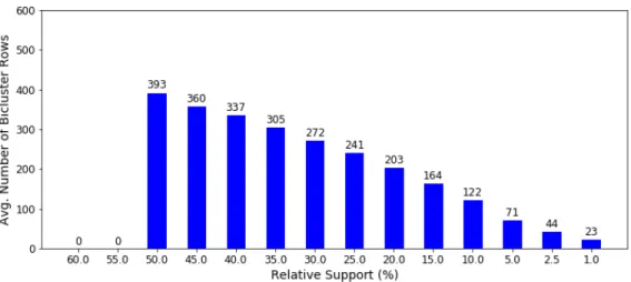
4.1 Average Number of Bicluster Rows vs Relative Support Percentage[Link]. . . 51
4.2 Biclustering Solution Purity vs Relative Support Percentage[Link]. . . 52
4.3 Number of Total/Discriminative Biclusters vs Relative Support Percentage[Link]. . . 52
4.4 Number of Discriminative Biclusters per Class vs Relative Support Percentage[Link]. . 53
4.5 Top-30 Most Important Features - a) Baseline All Features for Task 1[Link]. . . 55
4.6 Top-30 Most Important Features - b) Baseline FS for Task 1[Link]. . . 56
4.10 Biclustering Solution Purity vs Relative Support Percentage[Link]. . . 64 4.11 Number of Total/Discriminative Biclusters vs Relative Support Percentage[Link]. . . 64 4.12 Number of Discriminative Biclusters per Class vs Relative Support Percentage[Link]. . 65 4.13 Top-30 Most Important Features - a) Baseline All Features for Task 2[Link]. . . 67 4.14 Top-30 Most Important Features - b) Baseline FS for Task 2[Link]. . . 68 4.15 Top-30 Most Important Features - c) Matrix Subject ID × Biclusters for Task 2[Link]. . 69 4.16 Top-30 Most Important Features - d) Merged Data for Task 2[Link]. . . 70
1.1 Feature sets from the ONWebDUALS dataset standardized questionnaires. . . 3
2.1 Model types and respective expressions for Biclusters with Constant Values. . . 10
2.2 Model types and respective expressions for Biclusters with Coherent Values. . . 10
2.3 Confusion Matrix. . . 20
2.4 Evaluation Metrics for Binary Classification (adapted from [22]). . . 21
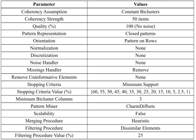
3.1 BicPAMS Parameters’ Description . . . 44
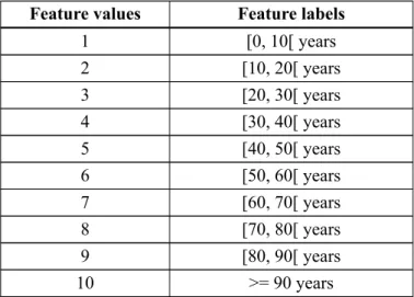
3.2 Example of feature translation from category values to category labels. . . 45
4.1 Descriptive Frequency Analysis per Class of Used Data for Task 1. . . 49
4.2 BicPAMS Parameter Values for Task 1. . . 50
4.3 Descriptive Analysis of Used Data Features for Task 1. . . 53
4.4 Evaluation Metrics for RF Classifier - 10-fold CV in Task 1. . . 54
4.5 Top-5 Most Important Bicluster Patterns - c) Matrix Subject ID × Biclusters for Task 1. . 58
4.6 Top-5 Most Important Bicluster Patterns - d) Merged Data for Task 1. . . 60
4.7 Metrics of Class Association Rule Mining experiments for Task 1. . . 60
4.8 Most Relevant Class Association Rules for Task 1. . . 61
4.9 Descriptive Frequency Analysis per Class of Used Data for Task 2. . . 62
4.10 BicPAMS Parameter Values for Task 2. . . 63
4.11 Descriptive Analysis of Used Data Features for Task 2. . . 65
4.12 Evaluation Metrics for RF Classifier - 10-fold CV in Task 2. . . 66
4.13 Top-5 Most Important Bicluster Patterns - c) Matrix Subject ID × Biclusters for Task 2. . 69
4.14 Top-5 Most Important Bicluster Patterns - d) Merged Data for Task 2. . . 71
4.15 Examples of Bicluster patterns for Neutral class - d) Merged Data for Task 2. . . 72
4.16 Metrics of Class Association Rule Mining experiments for Task 2. . . 72
2D Two-dimensional
AD Alzheimer Disease
ALS Amyotrophic Lateral Sclerosis
ALSFRS-R ALS Functional Rating Scale (Revised)
API Application Programming Interface
ARFF Attribute-Relation File Format
ARM Association Rule Mining
AUC Area Under Curve
C9orf72 Chromosome 9 open reading frame 72
CAR Class Association Rule
CI Confidence Interval
CK Creatine Kinase
CSV Comma-Separated Values
CV Cross-Validation
DM Data Mining
DMD Discriminative Meta-features Discovery
DT Decision Tree
EHR Electronic Health Record
EM Expectation-Maximization
EMG Electromyography
ENCALS European Network to Cure ALS
ESCO European Skills/Competences, qualifications and Occupations
fALS Familial ALS
FIM Frequent Itemset Mining
FN False Negatives
FNR False Negative Rate
FP False Positives
FPR False Positive Rate
FS Feature Selection
GUI Graphical User Interface
HDL High Density Lipoprotein
JPND Joint Programme - Neurodegenerative Disease
LDL Low Density Lipoprotein
LMN Lower Motor Neuron
MAR Missing at Random
MCAR Missing Completely at Random
MCC Matthews Correlation Coefficient
ML Machine Learning
MRI Magnetic Resonance Imaging
MS Multiple Sclerosis
NEUROCLINOMICS2 Unravelling Prognostic Markers in NEUROdegenerative diseases through CLINical and OMICS data integration
NIV Non-Invasive Ventilation
NMAR Not Missing at Random
NP Non-deterministic Polynomial (problem)
NSAID Nonsteroidal anti-inflammatory drug
ONWebDUALS ONTology-based Web Database for Understanding ALS
PD Parkinson’s Disease
ROC Receiver Operating Characteristic
SNIP Sniff Nasal Inspiratory Pressure
TN True Negatives
TNR True Negative Rate
TP True Positives
TPR True Positive Rate
TSV Tab-Separated Values
TXT Text File
UMN Upper Motor Neuron
Introduction
1.1
Context and Motivation
The work described in this thesis was done in the context of the NEUROCLINOMICS2 (Unravelling Prognostic Markers in NEUROdegenerative diseases through CLINical and OMICS data integration, with Ref. PTDC/EEI-SII/1937/2014) project at the LASIGE Research Unit (Ref. UID/CEC/00408/2019). This project’s main objectives are to understand Amyotrophic Lateral Sclerosis (ALS) disease progres-sion patterns and predict prognostic markers for personalized medicine. In this thesis we focused on the discovery of disease presentation patterns.
ALS is a heterogeneous neurodegenerative syndrome which affects the human motor system in a rel-atively short time period. Common symptoms are limb weakness, speaking and swallowing impairment, respiratory insufficiency and cognitive/behavioural changes. Eventually it culminates in respiratory fail-ure, which is appointed as the main cause of death. Survivability is highly variable, depending on the speed of disease progression [12,32].
To this day, it remains crucial to unravel definite diagnostic tests or biomarkers to help clinicians make a fast and clear diagnosis for this disease, given the high degree of variability in phenotype, family history, genes involved, molecular pathways and environmental factors that might induce it. Thus, it is believed that distinct mechanisms cause the neurodegeneration in ALS patients [32].
In this context, the use of Machine Learning models able to unravel the complexity of disease pre-sentation patterns is paramount for disease understanding, targeting improved patient care and longer survival times. Furthermore, explainable models are vital, since clinicians must be able to understand the reasoning behind a given model’s result or prediction before making a decision that can impact a patient’s life. [8].
1.2
ONWebDUALS dataset
The JPND ONWebDUALS two-dimensional dataset is the result of a collective effort from ENCALS, a consortium composed of partners from European countries. This dataset is the first in Europe to contain answers of standardized patient questionnaires of ALS patients and controls, regarding their demograph-ics, lifestyle, genetic mutations, family occurrences of ALS (or similar neurodegenerative diseases) and more. The major motivations behind the compilation of this dataset were to investigate the interplay between demographics, genetic mutations, clinical features and survival to discover causal relationships linking the patients’ specific risk factors and ALS genotype-phenotype [49,12]. So far, the dataset in-cludes information from Patients and Controls from four European countries (Turkey, Germany, Portugal and Poland) or, more concretely, five different cities (Antalya, Hannover, Jena, Lisbon and Warsaw).
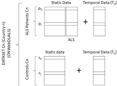
The data considered for each subject (Patient or Control) can be seen as:
- a set of static features (which could not change over time), which includes the information about the subject’s demographics, disease severity, co-morbidities, medication, genetic information, habits, trauma/surgery information and occupations;
- a set of temporal features (which could change over time), such as disease progression rate (e.g. ALSFRS-R scale measurements, pulmonary function tests measurements) and clinical laboratory investigations.
Considering what was aforementioned, the general layout of the data can be seen inFigure 1.1:
Figure 1.1: Layout of the ONWebDUALS dataset.
However, regarding the temporal features, it is important to state that a single time point (shown as a temporal snapshot T0 inFigure 1.1) was available in this dataset, thus being the only one considered.
is that disease-related features are specific to the ALS Patients (not being present in the Controls’ data). This can also be seen inTable 1.1, where the feature sets from the questionnaires are reported.
Feature Set Patients Controls
Demographic Information Yes Yes
Disease Features Yes No
Clinical Signs Yes No
Disease Severity and Progression Rate Yes No Investigations (laboratorial) Yes No Co-morbidities (other diseases) Yes Yes
Medication Yes Yes
Genetic Information Yes Yes
Habits / Trauma and Surgery Yes Yes
Occupations Yes Yes
Table 1.1: Feature sets from the ONWebDUALS dataset standardized questionnaires.
The analysis in this thesis is the first performed over this data, therefore special considerations had to be had in handling and cleaning the data. An exploratory analysis performed on the original dataset (over 600 features) revealed some issues: some features had irrelevant or erroneous values that needed to be treated or uniformized before discretization and others had duplicate column names. In addition, only Patients and Controls selected in Lisbon (472 Patients and 300 Controls) were considered for further analysis. This was done for several reasons: the Portuguese subjects were followed by one of our expert clinicians, having less missing information per subject and less prone to biases.
The entire data treatment performed is thoroughly detailed in Section 3.1.1 Data Pre-processing. The number of effectively considered features varied with the task and respective experiment, which are thoroughly described in Chapter 4 Discriminative Meta-features Discovery: A Case Study in the Portuguese ONWebDUALS Dataset.
1.3
Objectives and Contributions
The main objective of this thesis is to unravel disease presentation patterns of ALS patients on Electronic Health Record (EHR) data from the aforementioned ONWebDUALS dataset. These patterns can be found in the form of relevant subsets of features and their values (Meta-features), which caracterize and discriminate class-labeled two-dimensional data.
This main objective encompasses two clinical problems we tried to address as secondary goals. The first goal is to help improve diagnosis of the disease, to start the patients’ treatments as early as possible.
And the second goal is to help with the prognosis of ALS patients to help assess disease progression, refine therapeutical trial design and improve patient care.
To accomplish these goals, in this thesis is suggested a new Data Mining approach called Discrimi-native Meta-features Discovery (DMD). To the best of our knowledge, this approach uniquely combines Data Mining and Machine Learning techniques in order to find class-discriminative patterns in two-dimensional data. At its base is a specialised pattern-based Data Mining technique called Biclustering, which was used to identify any potentially relevant subsets of features (and their respective values) in this complex two-dimensional dataset. Up-to-date this technique has been successfully applied in healthcare data, allowing the discovery of groups of biological entities or individuals meaningfully correlated on a subset of conditions [44].
More concretely, the DMD approach is a workflow composed of several steps. First of all, the data is pre-processed (including discretization and class-labelling). Then Pattern Mining-based Biclustering is applied to the pre-processed data to find discriminative Biclusters and their patterns. Finally, the pat-terns from the Biclustering phase are further processed in two separate ways (using Biclustering-based Classification and Class Association Rule (CAR) Mining) to find the most discriminative Meta-features. Finally, in the context of this thesis the DMD approach was applied to the Portuguese portion of the ONWebDUALS dataset, where the aforementioned secondary goals were translated into concrete Tasks with distinct investigation directions:
1. Discover Meta-features which best distinguish the ALS patients from their controls, if any; 2. Discover Meta-features which caracterize ALS patients’ progression groups, if any.
1.4
Thesis Outline
This thesis is organized as follows. Chapter 2 Background and Related Workcontains all the background information, including a thorough disease description, important definitions and related work. Chapter 3 Discriminative Meta-features Discoveryfocuses on outlining the newly suggested DMD approach that was used to complete each one of the defined tasks. Chapter 4 Discriminative Meta-features Discovery: A Case Study in the Portuguese ONWebDUALS Datasetreveals the results of the performed experiments. Finally,Chapter 5 Conclusions and Future Work disclosures this thesis’ main conclusions and suggests possible future work.
Background and Related Work
2.1
Amyotrophic Lateral Sclerosis
Amyotrophic Lateral Sclerosis (ALS) is an idiopathic and heterogeneous neurodegenerative syndrome, which affects the upper and lower human motor system. The onset area of the body where the neurode-generation starts may vary, but within weeks or months progressive motor deficits ensue, difficulting proper nutrition and causing cognitive and/or behavioural changes. Eventually it culminates in respira-tory failure, appointed as the main cause of death. Survivability is highly variable, with the most common case being around 3-4 years, depending mostly on the origin onset area of the body and speed of disease progression [13,32].
ALS is usually classified in two main forms: familial (fALS) and sporadic (sALS). Familiar ALS comprises 5-10% of the cases, and it is the best understood form of the disease, since more than 30 genes and loci of major effect involved are, as of date, identified. The most frequent gene mutations occur on C9orf72, SOD1, FUS and TARDBP (which codes for the TDP-43 protein) genes. Sporadic ALS includes the remaining 90% of the patients. Even though it is the most frequent type, so far it has been difficult to concretely identify the underlying causes, since only 15% of the sALS cases can be explained by genetic factors. The only established risk factors are advanced age, male gender and some very specific genetic mutations [13,34].
Environmental factors have been proposed to explain the high prevalence of ALS in certain popula-tions, like smoking, exposure to pesticides and organic toxins, electromagnetic radiation and high levels of exercise. However, only smoking was proven to have a definite evidence of risk. Studies of relevant sample size are direly needed to test additional factors, such as dietary habits (fat and glutamate rich diets), gut microbiome and psychological stress [13,34].
(95% CI 2.0 to 2.3). Genderwise, for men the incidence rate is higher (3.0 per 100000 person years, 95% CI 2.8 to 3.3) than among women (2.4 per 100000 person years, 95% CI 2.2 to 2.6). These rates tend to increase with the advance of age for both genders, more pronouncedly after 40 years of age, reaching its apex at 70-74 years for men and 65-69 years for women. After that, disease occurrence declines rapidly [42].
On a more global scale, it has been proposed that different genetic etiologies underlying motor neu-ron degeneration may exist across major ethnic groups. One example of such was found in Japan, where OPTN gene mutations have been appointed as responsible for autosomal recessive ALS in Japanese fam-ilies [57].
The El Escorial criteria is used to diagnose patients who have a history of progressive muscle weak-ness that has spread to one or more regions of the body, and that any other disease cannot explain. Its final result is a degree of probability that the patient has ALS: definite, probable, probable (laboratory-supported) and possible [13].
To assess functionality and accurately track progression of patients’ disability, the Revised ALS Func-tional Rating Scale (ALSFRS-R) is used. This scale is composed of 12 questions, where each one can be evaluated in a scale from 0 to 4, totalling to a maximum of 48 points (indicating no dysfunction). This scale takes not only limb and bulbar function in consideration, but also the degree of respiratory disfunction, allowing a good evaluation of patients’ quality of function and life [7].
Additionally, it was recently discovered that ALS shares pathobiological features (e.g.: toxic aggre-gates of TDP-43 protein) with Frontotemporal Dementia (FTD), generating a whole spectrum of disease phenotypes in between. Some patients even tend to suffer from both conditions at once, or have someone in their family which suffers from one of the two [13].
Regarding possible treatments, currently the only widely available drug known to prolong ALS pa-tients’ survival is Riluzole, shown to increase life span for approximately 3 months. To alleviate the respiratory symptoms, Non-Invasive Ventilation (NIV) is commonly advised, since it extends survival with an effect size greater than Riluzole (median survival increase of 7 months), especially if started as soon as muscle weakness is detected [13].
In the last decades many technological advances have sped up the discoveries regarding this disease, but it remains crucial to unravel definite diagnostic tests or biomarkers to help clinicians make a fast and clear diagnosis. In addition, this would greatly help to assess disease progression, refine therapeutical trial design and start the patients’ treatments as early as possible [32].
In conclusion, taking into consideration the high degree of variability in phenotype, family history, genetic mutations, molecular pathways and possible environmental factors involved, it is believed that different mechanisms cause the neurodegeneration in ALS patients [13].
2.2
Unsupervised Learning
unsu-pervised due to the inexistence of a class label for each element of the dataset (no ground truth), such as Clustering, Biclustering and Pattern Mining. These techniques are widely used in Data Mining to group data observations based on their features’ values [22].
2.2.1 Clustering
Given a dataset with n observations, X = {x1, . . . , xn}, the Clustering task aims to find subsets of
observations (Clusters), {I1, . . . , Ir}, where every Ii ⊆ X satisfies certain intra-cluster (within a
Clus-ter) and inter-cluster (between different Clusters) criteria of (dis)similarity over the whole space [28]. A Clustering example is shown inFigure 2.1.
Figure 2.1: Illustrative example of Clustering.
Clustering can help discover previously unknown groupings within a dataset, and currently it is used in a myriad of very different applications (e.g. business intelligence, biology, image pattern recognition, web search and security). From a Data Mining point of view, it can be used as a standalone tool to retrieve new knowledge about and from the data, but it can also be used as a pre-processing step for other algorithms like classifiers. In extremis, a Cluster can be also seen as an implicit class: the objects in a Cluster are similar to each other and, at the same time, are different from the objects in other Clusters, which allows for automatic classification. Finally, it can also be used for outlier detection [22].
2.2.2 Biclustering
A two-dimensional (2D) dataset (or matrix) can be defined by n observations (rows) X = {x1, . . . , xn},
m attributes (columns) Y = {y1, . . . , ym}, and n × m elements (values) aij. Given a real-valued or
symbolic matrix A, the Biclustering task’s objective is to find a set of Biclusters B = {B1, . . . , Bq} (a Biclustering solution), such that each Bicluster Bisatisfies specific criteria of homogeneity and
statisti-cal significance [28].Figure 2.2shows an example of a Biclustering solution.
A Bicluster B = (I, J ) is a subspace given by a subset of rows I ⊆ X which show a coherent pattern observed for a subset of columns J ⊆ Y . It is considered maximal if and only if there is no other Bicluster B0 = (I0, J0) such that I ⊆ I0 and J ⊆ J0, while B ∈ {B1, . . . , Bq} and B0 ∈ {B1, . . . , Bq},
Figure 2.2: Illustrative example of a Biclustering solution.
The homogeneity criteria determines the structure, coherence and quality of a Biclustering solution, where it can be said that:
- The structure is described by the number, size, shape and position of said Biclusters (Figure 2.6); - The coherence of a Bicluster is defined by the observed correlation of values (correlation
assump-tion) and the allowed deviation from expectations (coherence strength);
- The quality of a Bicluster is defined by the type and amount of tolerated noise (values or symbols that differ from the expected pattern) and missing elements.
Taking these points into consideration, it sounds reasonable that the homogeneity criteria to apply to a given dataset should depend on its regularities: the possible domain of the dataset’s features - either if they are real-valued, symbolic or non-identically distributed - and their respective distribution [28].
To guide the search for Biclusters, a Biclustering algorithm uses a merit function, which evaluates how good a found Bicluster is based on the values of its elements. The chosen merit function is highly correlated with the characteristics of the Biclusters it can obtain, since it defines the type of homogeneity being sought in each one of them. It is important to use a different type of merit function to evaluate the quality of the identified Biclusters, in order to avoid evaluation biases [44, 28]. It is of note that
pattern-based merit functions exist, allowing to assess the maximality of Biclusters with well-defined
patterns composed of a set of symbols from one dimension, repeated over the other. These functions accommodate principles from Biclustering to handle non-constant patterns, sparse data and to minimize the drawbacks of discretization procedures (e.g. loss of information) by alleviating noise [28,25,65].
A Bicluster is statistically significant if its probability of occurrence deviates from expectations, that is to say that the found pattern has a very low probability of occurring by chance in the given dataset. To derive such a conclusion for a given Bicluster, the p-value probability from a statistical hypothesis test against a null data model is usually used [28]. In the same way as homogeneity, the statistical significance criteria to apply to a given dataset should depend on its regularities. Any Biclusters found must be subject to statistical assessments in order to:
1. Measure and minimize the risk of including irrelevant Biclusters in the solution (false positives, error of type-I);
2. Guide the Biclustering task without increasing the risk of excluding relevant Biclusters (false
neg-atives, error of type-II) [28,24].
However, even though this criterion is majorly important to guarantee the soundness of a given Bi-clustering solution, there is no agreed ground truth on how to verify and promote it. Many algorithms are guided by merit functions that enforce homogeneity over statistical significance, but having the former does not imply the existence of the latter, since it is very common for small Biclusters to have good ho-mogeneity levels by chance. Therefore, both criteria need to be combined and considered when choosing between solutions [28,24].
Besides what was said above for quality, it is important to underline that some actions included in the pre-processing (normalization and discretization) and post-processing (merging, filtering, extending and reducing) phases contribute for Bicluster quality adjustment to account for noise [28]. Moreover, some algorithms and frameworks have imputation procedures or dedicated interpretations to deal with missing values [18,27].
2.2.2.1 Types of Biclusters
Typically each subspace problem to solve has its own specificity, thus different types of Biclusters may be needed or considered interesting. The type of found Biclusters depends on the Biclustering algorithm and possibly its parameterization. As defined in [44], these different types can be categorized in four major classes: 1) Biclusters with constant values, 2) Biclusters with constant values on rows or columns, 3) Biclusters with coherent values and 4) Biclusters with coherent evolutions. Figure 2.3shows some examples:
2.2.2.2 Biclustering Models
At the basis of the aforementioned different types of Biclusters stand mathematical models which describe them and define their coherence.
Regarding Constant Valued Biclusters, they’re considered perfect if the Bicluster is a subspace (I, J ) where all real-valued elements aij are equal for all i ∈ I and all j ∈ J : aij = µ. An example of
this is given inFigure 2.3 a). However, since real data usually has noise, perfect Biclusters are rare to find. This means that a regular Constant Bicluster is better defined by aij = µ + ηij, where ηij is the
noise amount associated with the real value µ of aij [44].
When looking at Biclusters with Constant Values on Rows or Columns, we can have two types of models: Additive or Multiplicative, depending on the relation between the values. These Biclusters are considered perfect if the Bicluster is a subspace (I, J ) where all elements aij are obtained using one of
the following expressions:
Model Type Expression
Additive on Rows aij = µ + αi
Multiplicative on Rows aij = µ × αi
Additive on Columns aij = µ + βj
Multiplicative on Columns aij = µ × βj
Table 2.1: Model types and respective expressions for Biclusters with Constant Values.
where αi is the adjustment value per row i ∈ I and βj is the adjustment value per column j ∈ J .
Examples for the Additive case can be found inFigure 2.3 b) and c), by adding one unit either in the rows or the columns, respectively. By adding the noise parcel as before we get the regular versions of these Biclusters [44].
If the Additive and Multiplicative models were used to obtain Biclusters on both rows and columns at the same time, Biclusters with Coherent Values would be obtained. In the same fashion, for the perfect case we have:
Model Type Expression
Additive aij = µ + αi+ βj
Multiplicative aij = µ × αi× βj
Table 2.2: Model types and respective expressions for Biclusters with Coherent Values.
Examples of this model can be seen inFigure 2.3 d) and e), with the respective increments in grey for each row/column. The addition of the noise amount can also be applied to this model as well, in order to find regular Biclusters of these types [44].
When dealing with the possibility of Bicluster Overlapping, it is fair to consider that the value of an element in the matrix may be composed of several layers, either in an additive or multiplicative way. This is formalized by the Plaid model, given by aij = PKk=0θijkρikκjk, where K is the number of layers
(Biclusters) and the value of θijkindicates the contribution of each Bicluster k specified by ρikand κjk,
both binary terms which represent the membership of row i and column j in Bicluster k, respectively. It is of note that this notation allows the representation of the previously specified models of Biclusters depending on the definition of θijk. For example, if θijk = µk, then the Plaid model would identify a set
of K Constant Biclusters.
From the Plaid model two more restrictive models can be derived: the General Additive Model (GAM) and the General Multiplicative Model (GMM) [44]. For the former, as defined above in the Plaid model, every element aij represents a sum of additive models each representing the contribution
of the Bicluster (I, J )kto the value of aij in case i ∈ I and j ∈ J . Examples of this can be seen in the
following figure:
Figure 2.4: Overlapping Biclusters with GAM (adapted from [44]).
For the latter, every element aij represents a product of contributions of the Bicluster (I, J )kto the
value of aij in case i ∈ I and j ∈ J . It means that in this case the value of each element is given by
aij =QKk=0θijkρikκjk. Equivalently, some examples are provided:
Figure 2.5: Overlapping Biclusters with GMM (adapted from [44]).
patterns. Those Symmetries are considered relevant in some areas (e.g. to find activation or repression mechanisms in regulatory processes on Gene Expression data), and can only be captured by Biclustering algorithms that support them [27].
Finally, the last kind of models that needs to be mentioned are the ones that find Biclusters with
Coherent Evolutions. These models permit to address the problem of finding coherent evolutions (or
trends) across the rows and/or columns of the matrix without regarding the exact value of the elements. Additionally, these models are the only ones that can be applied to symbolic/categorical data. Examples of this can be found inFigure 2.3 from f) to h)for categorical data andFigure 2.3 i)for real-valued data [44]. In this work we consider Biclusters with Coherent Evolutions to be the target since the data being processed by the algorithm is purely categorical.
2.2.2.3 Types of Bicluster Structures
Another important aspect is the Biclusters structure that a Biclustering algorithm is able to discover. In its simplest form, an algorithm will assume one of two things: that there is only one Bicluster in the data matrix, or that it contains K Biclusters, where K is the number of Biclusters expected to be found. If it is the latter case, according to Madeira et al. [44] several different types of structures within a set of Biclusters can be encountered:
Figure 2.6: Examples of different types of Bicluster structures (adapted from [44]).
Additionally,Figure 2.6 b) to e) presents structures which assume exhaustive Biclusters, in which every row and column in the matrix belongs to at least one Bicluster. However, most of the structures presented above are very restrictive. In real data, it is most probable that some rows and columns do not belong to any Bicluster and that Biclusters can overlap each other, like it is seen inFigure 2.6 i)[44]. Other stopping conditions besides the number of Biclusters to discover are also possible, which will be seen later
onChapter 3 Discriminative Meta-features Discovery. In this work we will use a Biclustering algorithm able to find arbitrarily positioned overlapping Biclusters (Figure 2.6 i)) since structure restrictions do not make sense in our problem.
2.2.2.4 Biclustering Evaluation
To define evaluation measures for Biclustering solutions, we need to distinguish two types of possible datasets:
1. Synthetic data, artificially generated data with planted Biclusters, used to test the accuracy of a given algorithm against a true and known solution (ground truth, also known as true or hidden Biclusters);
2. Real data, any dataset without a ground truth [28].
Solutions obtained from applying Biclustering algorithms to a given dataset will vary according to the chosen algorithm and its parameterization. Therefore, metrics to evaluate and compare said solutions are important to find the best algorithm, if an algorithm is working well or the best result between exper-iments. In this thesis we are interested in the last case. Evaluation metrics (or indices) can be divided in three main categories: external, internal and relative.
External metrics determine the similarity between an obtained solution and apriori knowledge, and
can be used with synthetic data (Accuracy-based views) or with real data plus additional domain informa-tion (Domain Significance views). In addiinforma-tion, they can be used to compare different algorithms. These are the most abundant type of metric and the ones usually preferred, since they have greater precision and are easier to define, use and implement [60].
Internal metrics contrast the obtained solution with the intrinsic structure of the dataset. These
met-rics have to be used when no ground truth is available, although they are not as precise as the external ones. However, they are usually adapted from Clustering concepts (e.g. Cluster compactness and sepa-ration) which are hard to extend when Bicluster overlapping is allowed. Therefore, when working with real data they tend to be avoided, mostly if there is a possibility of creating a synthetic dataset [60].
Relative metrics are used to compare different configurations of input parameters and solutions, in
order to find the optimal set of parameters for a given dataset. The usual procedure is to evaluate and rank each solution obtained from the different user-defined combinations of parameters to select the best. To obtain the best results, all combinations should be investigated. However, these metrics are very complex to formulate and thus almost non-existent, since Biclustering algorithms are very heterogeneous relatively to their input parameters [60].
Finally, if no usable metric exists, a possible alternative is to define a criteria of usefulness depending on the problem to solve and the characteristics of the Biclusters to find the best solution. In this thesis we used such a solution, by choosing the best Biclustering solutions according to the number of discrimina-tive Biclusters in them (as specified later in this document, inSection 2.3.2 Discriminative Biclustering and inSection 3.1.3 Pattern Mining-based Biclustering).
2.2.3 Clustering vs Biclustering
Regular Clustering solutions are limited to grouping objects one dimension at a time, by using all features that describe a given set of objects [28]. This means that they derive a global model from the data, which is a restriction when dealing with 2D data spaces with only locally correlated values [28,44]. This can be clearly seen inFigure 2.7below:
Figure 2.7: Clustering and Biclustering Comparison (adapted from [18]).
Data Mining techniques like Biclustering are then necessary to identify any potentially relevant sub-spaces in complex 2D datasets, as they can perform local clustering on both dimensions simultaneously (local model [44]). Additionally, groups of biological entities or individuals are usually meaningfully correlated only on a subset of conditions/records [28].
However, Biclustering is computationally expensive due to combinatorial optimization. Best case scenario, this task is an NP (Non-deterministic Polynomial) problem, meaning it is solvable in polynomial time, but it becomes more complex when searching for non-exclusive and non-exhaustive Biclusters. Due to this, most algorithms follow heuristics or stochastic approaches, by producing sub-optimal solutions or adding constraints to simplify the problem. Other approaches, such as Pattern Mining-based Biclustering, target exhaustive enumeration while using restrictions during the search for efficiency [25].
2.2.4 Pattern Mining
Consider a finite set of items L, and P as an itemset where P ⊆ L. One transaction t can be defined as a pair (tid, P ) with id ∈ N. A finite set of transactions {t1, . . . , tn} then composes an itemset database
D over L. If another itemset P0 ⊆ P , it implies that P0 ⊆ (t
id, P ). The coverage of an itemset P , φp, is
the set of all transactions in D where P occurs: φp = {t ∈ D | P ⊆ t}.
From this we can derive the support of P in D, supP, that can be either absolute (the size of φp,
| φp |) or relative (| φp | / | D |). More simply, the support is the frequency (absolute or relative) of
the itemset P in the database D [25].Figure 2.8below exemplifies the computation of the coverage and support of an itemset P over an itemset database D.
Figure 2.8: Example of an itemset database D with the coverage and support of an itemset P .
Given an itemset database D and a user-defined minimum support threshold θ, the Frequent Itemset
Mining (FIM) problem consists on the computation of the set {P | P ⊆ L, supP ≥ θ}. Thus, a Frequent Itemset or Pattern is an itemset P with supP ≥ θ. In simpler terms, an itemset is frequent if it appears in a dataset with a frequency equal or greater than the user-specified threshold [25].
A closed frequent itemset is a frequent itemset which has no superset with the same support. A
maximal frequent itemset is a frequent itemset for which all supersets are not considered frequent [25]. The closed frequent itemsets are a subset of the frequent, just like the maximal frequent are a subset of the closed frequent, as shown inFigure 2.9.
Figure 2.9: Frequent, closed frequent and maximal frequent itemsets.
FIM relies on monotonic and anti-monotonic properties to prune over combinations of itemsets in order to gain efficiency. Considering two itemsets P and P0, where P0 ⊆ P , and a predicate M , M is monotonic if M (P ) ⇒ M (P0) and anti-monotonic when ¬M (P0) ⇒ ¬M (P ). This means that the support of P is bounded by the support of P0, implying that if any subset P0 is not frequent, then P is not frequent as well [25].
Three major search strategies can be used to perform FIM:
1. Apriori-based, which applies the monotonicity principle (an itemset is candidate if all its subsets are frequent) to iteratively combine (k − 1)-itemsets to generate new candidate k-itemsets in k scans, until no new candidate groups can be found;
2. Pattern Growth, which builds a frequent-pattern tree from an ordered list of frequent items to be later mined, based on prefix paths co-occurring with growing suffix patterns;
3. Vertical projection, which compiles the set of transaction ids where each item appears and then grows the itemsets using a depth-first strategy, by intersecting the sets of transaction ids to minimize scanning the database [25].
The first two search strategies listed above consider itemset databases in the horizontal format: {tid, P }, where tid is the transaction id and P is the set of items involved in said transaction, as seen
inFigure 2.8. The last one considers the database is in the vertical format: {item : {tid1, . . . , tidn}}, where each item is associated with the set of transaction ids from the transactions where it appears [22].
2.2.5 Pattern-Mining based Biclustering
As aforementioned, traditional Biclustering algorithms use flexible merit functions to guide the data space exploration. However, constraints like searching for a fixed number of Biclusters or retaining only non-overlapping structures are put in place, to ease the problem’s complexity [25].
Pattern Mining-based approaches require the redefinition of those functions in terms of support and other relevant metrics, but in doing so they allow for a scalable exhaustive space search. This, in turn, produces a flexible structure containing an arbitrarily high number of Biclusters, while still catering for homogeneity and statistical significance criteria. These approaches can be divided in three major steps: mapping, mining and closing. All three steps are relevant in affecting the solution’s coherence, structure and quality [25,28].
The first step - mapping - is responsible for the normalization and discretization of the data matrix. Since the data has to be itemized to use Pattern Mining-based solutions, usually this step is mandatory for real-valued data. However, it can be optional if the algorithm is able to discretize the data internally or if the data is already discretized. In this phase it is also performed the handling of outliers, missing values and noisy elements. The second step - mining - is the core task, composed by the application of the target pattern miners that will model the type of Biclusters that can be found in the given solution. The last step - closing - deals with the post-processing of the mined patterns, to mostly improve the quality of the found solution. This is done through merging (affecting structure and dealing with overlapping while still maintaining homogeneity), extension (to improve noise tolerance) and filtering (to deal with Biclusters numerosity and compactness) [25].
2.2.5.1 Advantages and Disadvantages of Pattern Mining-based Biclustering
Pattern Mining-based approaches’ major benefits are: - Efficient exhaustive searches;
- Dealing with missing and noisy data;
- Ability to use different models to search for specific types of Biclusters; - Annotating the significance of Biclusters to assess the pattern’s relevance;
- Producing non-exhaustive, non-exclusive structures of Biclusters where overlapping is allowed. Thus, and in accordance with Henriques et al. [25], these approaches are well suited to find shared local patterns within physiological and clinical data. However, performing data discretization always im-plies some loss of information. In particular, when discretizing real-valued features, the items-boundary
problem can occur: assigning two elements with similar real-values to two different categories due to
their closeness to the interval boundary. To minimize this problem, multi-item assignments can be ap-plied: elements with values near a cut-off point of discretization can be assigned to the two categories associated with the closest ranges of values [25,24].
2.2.5.2 Meta-features
When using Pattern Mining-based Biclustering to look for Constant Biclusters on Rows or Columns ( Fig-ure 2.3 b) and c)) and Coherent Evolution on Rows or Columns (Figure 2.3 g) and h)) it is possible to discern a representative pattern of each real-valued or categorical Bicluster, respectively. These pat-terns are composed by subsets of features (and their respective values) which characterize a Bicluster’s contents. They can be seen as frequent patterns, representing a distinct data space with greater discrimi-native power than when considering only their constituent feature-value pairs individually, allowing them to capture additional underlying knowledge in the data [22,44].
In this thesis, when those patterns can characterize and discriminate class-labelled data they will be called Meta-features. For example, assuming features Fiwith i ∈ N on columns and observations on
rows, the pattern for the Bicluster in Figure 2.3 h)is {F1 = S1, F2 = S2, F3 = S3, F4 = S4}. By
finding the most class-discriminative Meta-features it is possible to unravel disease presentation patterns.
2.3
Supervised Learning
In Machine Learning, Supervised Learning includes all techniques whose learning process is con-sidered supervised due to the existence of a label for each element of the dataset (the ground truth that should be predicted), such as Classification (where a categorical class is being predicted) or Regression (where a numeric value is being predicted) [22]. In this thesis the focus is Classification.
2.3.1 Classification
Classification can be defined as the process of finding a model that describes and distinguishes data
classes or concepts. Such models, called Classifiers, are used to predict categorical/symbolic class labels for new observations, and are constructed in two phases:
1. The Training phase, where the Classifier is built by learning from the Training data: the model internally defines at least one decision boundary from the data features, as seen inFigure 2.10;
2. The Test phase, where the trained Classifier is evaluated with the remainder (and unseen by the model) Test data [22].
Figure 2.10: Illustrative example of a decision boundary on a Binary Classification problem. For Classification, the used datasets must be composed of observations/tuples and their associated class labels. A tuple X is an n-dimensional feature vector, X = (x1, x2, . . . , xn), which contain its n
feature values [22]. For example, the dataset’s data tuples forFigure 2.10should contain the values for their two features (f1 and f2), and each tuple must also have a class label (cat or dog).
Classification problems can be divided according to the number of classes found on the dataset: with only two class labels it is a Binary Classification problem (as seen inFigure 2.10); when there are more than two class labels it is considered a Multiclass Classification problem. Multiclass Classification problems are more complex than the Binary (they can have several decision boundaries), and many real-world problems are of the former kind [40].
2.3.1.1 Classifier Example - Decision Trees
In this section, a representative Classifier model - Decision Trees - which supports Binary and Multiclass Classification is introduced. Decision Trees (DTs) are widely used models in Data Mining and Machine Learning, due to being easy to understand, visualize and interpret [29]. The majority of algorithms that build a DT from the Training data (e.g. ID3 [52], C4.5 [53] and CART [3]) employ a greedy top-down recursive divide-and-conquer strategy: the data is recursively divided into smaller partitions by selecting in each iteration the feature which separates best the data tuples into their respective classes (the splitting
attribute), by using an attribute selection measure (e.g. Information Gain [52], Gain Ratio [53] or Gini Index [3]). The objective of these measures is to obtain, as much as possible, pure partitions, where all tuples belong to the same class [22]. However, the Information Gain is biased in favor of categorical features with more levels, with the Gain Ratio being proposed to tackle this issue [10].
While running the algorithm, if after a split all the tuples in a partition belong to the same class, a leaf node is created and labeled with the said class. Otherwise, the remaining data is split again on the next feature that divides it best. Finally, if it reaches a point where there are no more features available on which to split any last tuples, the class for the last leaf is decided by majority voting (the most frequent class on those tuples) [22].
On the example seen inFigure 2.11, the splitting attributes are enclosed in rectangles, and the leaf nodes in ellipses. The root split also shows that a DT can have any number of children for each node. The partitioning scenarios depend on the type of feature being split: for categorical features usual cases are splitting by all categories or one-vs-rest, while for real-valued features thresholds are defined (e.g. A < 5 and A ≥ 5). After building the model, in order to classify a new tuple, the DT’s nodes are traveled from the root, following the branches according to the new tuple’s feature values until reaching a leaf node with a class. By travelling all tree branches a set/list of prediction rules can also be obtained [22].
Figure 2.11: Example of a Decision Tree built from the PlayTennis example dataset (adapted from [46]). DTs are suitable for Binary and Multiclass classification, particularly when the number of data fea-tures is not too large, since they tend to overfit [54]. To minimize this, strategies like pruning to remove less informative branches can be applied. Moreover, the DTs construction strategy implicitly selects the most important data features, since the features which better split the data space appear higher on the tree (or in the tree at all) [22].
2.3.1.2 Model Selection and Evaluation
Classifier Performance Evaluation Metrics
The construction of a Classification model tends to be an iterative process, hence justifying the need of the Test phase. Without proper validation the model might not be able to correctly predict the class label of new observations, rendering it less useful than it could be. In a Classification problem there are two types of tuples: Positive tuples, the tuples from the main class of interest; and Negative tuples, the tuples from the remanining classes [22]. Based on this, it is possible to further compute the intermediate components of evaluation measures:
- True Negatives (TN): number of Negative tuples correctly labeled;
- False Positives (FP): number of Negative tuples incorrectly labeled (type-I errors); - False Negatives (FN): number of Positive tuples incorrectly labeled (type-II errors) [22]. These four terms are usually condensed in a tabular form, called a Confusion Matrix (Table 2.3),
Predicted class
Positive Negative Total
Actual class Positive T P F N P
Negative F P T N N
Total P0 N0 P + N
Table 2.3: Confusion Matrix.
where the actual Positive and Negative tuples are identified as P and N , respectively. In similar fash-ion, P0 and N0 identify the tuples predicted as Positive and Negative by the model. Taking this into consideration,Table 2.4characterizes some of the most usual evaluation metrics.
Metric Formula Description
Accuracy, Recognition Rate
T P +T N P +N
Percentage of Test set tuples correctly classified
Error Rate,
Misclassifica-tion Rate
F P +F N P +N
Percentage of Test set tu-ples incorrectly classified (1 - Accuracy)
Recall, Sensitivity, True Positive Rate (TPR)
T P P
Proportion of Positive tu-ples that are correctly clas-sified
Specificity, True Negative
Rate (TNR)
T N N
Proportion of Negative tu-ples that are correctly clas-sified
False Negative Rate
(FNR), Miss Rate
F N P
Proportion of Positive tuples that are incorrectly classified (1 - Recall)
False Positive Rate (FPR),
False Alarm Rate
F P N
Proportion of Negative tuples that are incorrectly classified (1 - Specificity)
Precision T PP0
Percentage of tuples cor-rectly classified as Positive
![Figure 2.6: Examples of different types of Bicluster structures (adapted from [44]).](https://thumb-eu.123doks.com/thumbv2/123dok_br/18270447.880640/35.892.171.729.610.875/figure-examples-different-types-bicluster-structures-adapted.webp)
![Figure 2.11: Example of a Decision Tree built from the PlayTennis example dataset (adapted from [46]).](https://thumb-eu.123doks.com/thumbv2/123dok_br/18270447.880640/42.892.116.788.359.601/figure-example-decision-tree-playtennis-example-dataset-adapted.webp)