National Borders and Conservation: Evidence from
the Amazon
Robin Burgess
∗Francisco J. M. Costa
†Benjamin A. Olken
‡March 30, 2017
Abstract
Tropical deforestation is one of the major drivers of climate change. Much of this loss is due to illegal logging. Unlike forests in the Congo basin and South-East Asia, the world’s largest tropical forest - the Amazon - has experienced a dramatic slowing in rates of deforestation over the last decade. The bulk of the Amazon is located in Brazil which has introduced a raft of policies to reduce illegal logging in recent years. We use Brazil’s border with its neighbors to identify the impact of Brazilian policies on deforestation. Because forests are a fixed resource and geography and infrastructure vary continuously over the border we can compare annual forest loss on either side of the border to tease out the impact of national forest policies from other drivers of deforestation. To do this we employ a satellite-derived data set that measures forest cover at a 30 x 30 meter resolution for the entire Amazon area across the 2000-2014 period. Our data reveals a sharp discontinuity at the border – in 2000 Amazonian pixels on the Brazilian side of the border are more likely to have been deforested and between 2001 and 2005 annual forest loss in Brazil was around four times the rate on the other side of the border. However, in 2006, just after the Brazilian government introduced a raft of policies to curtail illegal logging, these differences disappear and Brazilian rates of forest loss fall to those observed across the border. These results demonstrate the power of the state to affect whether or not natural resources are conserved or exploited even in the furthest reaches of the Amazonian jungle.
We would like to thank João Amaro, Gabriel Mesquita and Christiane Szerman for excellent research assistance. Francisco Costa gratefully acknowledges financial support from Rede de Pesquisa Aplicada FGV.
∗London School of Economics. E-mail: [email protected].
†Getulio Vargas Foundation (FGV/EPGE). E-mail: [email protected]. ‡MIT. E-mail: [email protected].
1
Introduction
Avoiding catastrophic climate change is a central challenge for the 21st century. Preser-vation of tropical forests has been identified climate as critical in this respect. These forests, which cover large swathes of the tropics, capture carbon from the atmosphere and play a central role in determining the pace of climate change. Because climate change does not recognize national borders and will affect humans everywhere the preservation of tropical forests is an international policy priority, and large amounts of resources are being channeled worldwide to the small number of countries in which these forests are located.1
Set against this growing realization of the importance of preserving this global resource is the hard reality that tropical deforestation has actually been accelerating in recent years (Hansen et al., 2013). The main reason for this is illegal deforestation. In the weakly institutionalized settings of developing countries there is often a large gap between de jure and de facto forestry policy. Policy enforcement is typically very weak and those interested in deforestation, whether to harvest timber or use the land for other purposes, often collude with local politicians and bureaucrats to circumvent official rules and regulations (Burgess et al., 2012). The result is that timber is often extracted from illegal sources and overall rates of extraction are more rapid than is officially sanctioned. This equilibrium where illegal deforestation benefits the few at the cost of the many has proven to be highly resilient.
When we view the earth from space three big areas of tropical forest are visible. The first (and largest) area is the Amazon which is mainly in Brazil. The second main area is the Congo basin which is mainly in the Democratic Republic of Congo (DRC). The third main area is in South-East Asia and is mainly in Indonesia. Figure 1 plots annual rates of forest loss (i.e. the change in forest cover) for Brazil, DRC and Indonesia from 2001 to 2014. Brazil is shown to be experiencing more rapid deforestation than DRC and Indonesia in 2001, but deforestation rates begin to fall in 2005. In contrast DRC and Indonesia experience rising deforestation rates from 2001 onwards with rates roughly doubling in both countries between 2001 and 2014. The net result is that Brazil starts the period with highest rate of deforestation and ends it with the lowest rate of deforestation. While Brazil comprises the majority of the Amazon land area, 35 percent of the Amazon is actually located in other South American countries – Bolivia, Peru, Columbia, Venezuela, Guyana, Suriname, and French Guyane. In Figure 2 we focus on deforestation in the Amazon and break it into two sections - that located in Brazil and that located neighboring countries. This reveals that the decline in deforestation in the Amazon that began in 2005 observed in Figure 1 is unique to Brazil. In contrast, deforestation rates
1The Norwegian Government, for example, has pledged $1 billion each to Brazil and Indonesia to
in non-Brazilian Amazon grow steadily from 2001 and have almost doubled by 2014 thus mirroring the pattern seen in DRC and Indonesia.2 This suggests that something changed in Brazil in the mid 2000s which caused the rate of forest loss to dramatically slow down. This paper asks whether the decline in deforestation in Brazil was due to specific forestry policies introduced by the Brazilian government, or whether it was caused by changes in the myriad other drivers of deforestation, such as roads and transportation costs (Pfaff, 1999; Barber et al., 2014; Souza-Rodrigues, 2015), commodity prices or other changes in soy and beef markets (Nepstad et al., 2006; Assunção et al., 2015), changing geographic patterns of complementary economic activity (Hargrave & Kis-Katos, 2013), and so on.
To do this we employ a novel identification strategy where we use detailed Landsat satellite data from Hansen et al. (2013) to measure deforestation on either side of Brazil’s border with its eight neighbors which together make up the Amazon region. The borders are porous and poorly maintained, allowing free flow of people and goods (Alston et al., 2012; Raza, 2013).3 Because forest is a fixed resource, and because we can demonstrate that geography (slope, distance to water) and infrastructure (distance to roads, distance to urban center) vary smoothly across the Brazilian border, we argue that we can interpret discontinuous changes in deforestation rates around the border as capturing the influence of national forestry policies.
When we examine the 30 x 30 meter forest cover data within a narrow strip on either side of the border we find that, in 2000, forest cover is significantly lower on the Brazilian side of the border.4 This may reflect both limited enforcement of forestry policy and the cumulated impact of policies to open up and develop the Brazilian Amazon. Consistent with this we find that Brazil is deforesting the Amazon forest at around four times the rate of its neighbors up to 2005. However, from 2006 onwards, deforestation rates in the Brazilian Amazon fall precipitously down to the levels observed in Brazil’s neighbors. Looking at these narrow strips of pixels along the Brazilian border we see that the gap in deforestation rates between Brazil and its neighbors disappears in 2006.
This is a striking finding and we find that this coincides with a major shift in forestry
2Though it is notable that deforestation rates in the non-Brazilian Amazon remain lower than those
in DRC and Indonesia.
3Indeed, the borders are so porous that in 1994, Brazilian President-Elect Cardoso, on vacation near
the border, accidentally wandered into Bolivia, spending over an hour before being stopped by a Bolivian solider. The solider reported that Cardoso was the first person he had ever stopped crossing the border (Cardoso & Winter, 2007).
4We restrict our analysis to pixels close to the border – using the Imbens & Kalyanaraman (2012)
optimal bandwidth criterion, we focus on a bandwidth of only 17 km on either side of the border, though we find results even when restricting ourselves to looking at bandwidths only 5 km on either side of the border. Other than a small section of the northern border with Venezuela, which is coincident with a mountain ridge, we find that observable characteristics such as slope, distance to urban areas, water, and roads are similar on both sides of the border. Results hold even when we control separately for distances to Brazilian and non-Brazilian infrastructure separately.
policy in Brazil. As it has been documented before (Nepstad et al., 2009; Assunção et al., 2013b,a), starting in 2004 the federal government launched the Action Plan for the Prevention and Control of Deforestation in the Legal Amazon (PPCDAm). This was a wide ranging policy reform that proposed several actions focused mostly on territorial and land planning along with strengthening the specific legislation and the environmen-tal monitoring and control. Although PPCDAm was released in 2004, its actions were implemented gradually; in particular, 2006 is exactly the year when Brazil promulgates the Law on Public Forest Management and when the Environmental Agency’s Center for Environmental Monitoring (CEMAN) became fully operational (MMA, 2008).
The appointment of Marina Silva in 2003 (an environmental activist who is from the Amazon) to be Minister of the Environment led to dramatic shift in forestry policy.5 The work of different agencies and ministries involved in environmental protection were now coordinated and satellite images were intensively used to detect illegal logging. Once de-tected both the army and federal police were deployed to arrest individuals and confiscate machinery. Legal changes and improved monitoring and enforcement severely blunted incentives for individuals and firms to be involved in illegal logging. Though a range of factors from wood prices (which affect demand) to transportation infrastructure (which affect supply) can affect rates of deforestation, the patterns we observe around the Brazil-ian border are consistent with us capturing changes in the forestry policy environment in Brazil.6
We find that our results are robust to restricting our analysis to artificial borders as in Alesina et al. (2011) – i.e. those which are literally straight lines drawn on a map, as opposed to following natural features such as rivers. Also when we divide the Brazilian Amazon into protected areas and unprotected areas we find that the main reversal in deforestation rates is occurring in unprotected areas. This pattern is consistent with enforcement of forestry policy strengthening from the mid 2000s onwards. We find that access to roads in Brazil encourages deforestation but that this effect is mitigated once new policies to protect the Brazilian Amazon are introduced. This suggests that proximity to roads is necessary for intense deforestation to take place, but it is not sufficient as enhanced enforcement of forestry policy can afford protection to accessible parts of the Amazon.
To quantify the magnitude of the border effects, we estimate a logit model on the Brazilian side of the border with Bolivia (where deforestation of the Amazon was con-centrated) that calculates the probability that each pixel was deforested in 2001 as a
5Marina Silva was the colleague of Chico Mendes an environmental activist and trade union leader
who was assasinated in 1988 by a cattle rancher in retaliation against his efforts to preserve the Amazon rainforest and protect the indigenous peoples that inhabit it.
6Timber and other commodities are a global market and so changes in prices for example should affect,
function of observable factors – such as slope, distance to water, to roads and to urban areas. This allows us to quantify the “Brazil effect” in terms of observables as we compare the propensity that each pixel on both sides of the border is deforested. We find that, until 2005, the pixels that were actually deforested on the Bolivian side of the border had on average around 25 percent higher propensity to deforest than those pixels deforested on the Brazilian side. Interestingly, this pattern reverts after 2005 and, by 2009, the average propensity to deforest of deforested pixels in Brazil and Bolivia become level. Therefore, it seems that unobservable factors - such as national forestry policies - were underlying the discontinuously higher annual forest loss on the Brazilian side on the border.
This paper contributes to the growing literature on the management of natural re-sources in developing countries. A key finding in this regards is that we show that the Brazilian state had the power to influence resource extraction rates even in the remotest part of its territory thus running contrary to a large literature in development that suggests that the state has limited reach in such remote areas (Herbst, 2000). It also contributes to the literature on using political borders to capture the influence of institutions and policies. The pathbreaking paper by Holmes (1998) examines changes in manufacturing across US state borders to examine whether pro-business regulations affect manufacturing activity. Michalopoulos & Papaioannou (2014) examine whether there is a change in lights at national borders in Africa to test whether national institutions matter. The challenge with these studies is that the estimates become hard to interpret if production or con-sumption can be easily relocated across the border. For example, imagine that businesses have only a slight preference for locating in a pro-business state. If capital and labor are all freely mobile across the border, businesses may simply relocate to take advantage of the regulations. Comparing the amount of business activity located on the pro-business side of the border to the amount on the other side would vastly overstate the true impact of the policy on the level of manufacturing activity, as it would be largely just picking up this relocation. On the other hand, comparing household incomes across the border might understate the impact of the policy: workers could all work in the high-productivity state but live on both sides. The same challenges occur in the African context where borders are porous and workers often freely cross back and forth each day. In this respect our analysis using a factor of production - trees - which is fixed in space helps to overcome some of these difficulties.
The remainder of this paper is organized as follows: in Section 2 we provide back-ground onthe recent trends in the Brazilian Amazon land use pattern, the Action Plan for the Prevention and Control of Deforestation in the Legal Amazon (PPCDAm), review the existing literature on deforestation in the Amazon and descibe and the data we em-ploy. We outline the details of our empirical method in Section 3, and we present results in Section 4. We draw conclusions in Section 5. The appendix contains supplemental
material, such as a brief timeline of PPCDAm.
2
Background and Data
In this section we describe the background of the recent trends in the Brazilian Amazon land use pattern, and the Action Plan for the Prevention and Control of Deforestation in the Legal Amazon (PPCDAm) implemented in mid-2000s to reduce the accelerated deforestation rates in the Brazilian Amazon. We then briefly describe the related literature and the data used in this paper.
2.1
Background
2.1.1 The formation of the Brazilian border
The broad limits of the Brazilian territory was defined in the colonial period when the Portuguese and the Spanish Crowns had very limited knowledge about the precise geog-raphy of the center of the South American continent. The Treaty of Madrid defined the general lines of the Portuguese – Brazilian – border with the Spanish colonies in 1750. Although the general limits of the colonies are not exogenous due to political and eco-nomic interests, we can interpret the precise location of border as locally exogenous in the Amazon area.
When drawing the Treaty of Madrid map, Portugal and Spain agreed on two general guidelines: (i) who had first established local presence should keep the area (uti possidetis); (ii) rivers should be used as border divisions as much as possible to easy demarcation. The main objective of Portugal during the negotiations was to hold the control of the (known) mining regions located between the center of the continent and the Atlantic coast, pushing the border West to keep potential invaders away. The main objective of the Spanish crown was to maintain navigable access to the sea. To make clear the interests involved during the negotiation, we break the Brazilian border in the Amazon area in two segments: the area dividing the limits with current days Bolivia and Peru, and the Northern segment of the border.
Regarding the first border segment, having departed from the coast in Rio de Janeiro and São Paulo and moving West, the Portuguese had explored most of the central region of Brazil by 1750. They found gold and other precious minerals in different regions as far West as the area around Cuiabá (the current capital of Mato Grosso state), but they did not find gold further West. In anticipation to the uti possidetis principle, the Portuguese had sponsored settlements in the areas they found valuable resources in order to guarantee the rights over it (Cintra, 2016). Since the Spanish Crown had found plenty of gold in its colonies, they did not give that much attention to that area. As a consequence, the
Treaty of Madrid set that the limits of the colonies in that region would be defined by the Paraguay and Guaporé Rivers, which are located more than 200km and more than 500km, respectively, from Cuiabá. In sum, while Spain guaranteed the territory to the West of Paraguay river important for navigation and access to the sea, Portugal guaranteed a 200km buffer from anywhere they knew had gold.
It is also worthy to have in mind that the geography of the center of the South American continent was still largely unknown in that time in the middle of the 18th century. This was particularly true for the Amazon area and the Northern segment of the Brazilian border. The magnitude of this “unknown” land can be seen by the vast blank spaces in the base map used in the Treaty of Madrid: Carte de l’Amérique Méridionale.7 The French cartographer Jean-Baptiste d’Anville made the map from Paris based on other maps, documents and diaries of explorers and priests of the time. The main source of information about the Amazon geography was the notes taken by the French explorer Charles Marie de La Condamine a member of the French Spanish-French Geodesic Mission to Quito. After losing the race to prove the shape of Earth, La Condamine decided to navigate through the Amazon River back to Europe in order to guarantee the mission a novel scientific contribution (Furtado, 2012).8 Information about the geography and resources available in the Amazon region was scant and mostly restricted to the land very close to its major navigable rivers. As a matter of fact, the precise location of rivers’ springs and mouths – and what was between them – was not exact. The straight line segments we can see in the Brazilian border are a consequence of this lack of information. These are due to rivers that followed a different path than the predicted one or that ended before reaching other geographic feature.9
It is important to highlight that there is one border segment which limits were defined under local pressure: the area corresponding to the Brazilian state of Acre, bordering Peru and Bolivia. In 1877, numerous Brazilian migrants started to occupy the area attracted by the boom in the rubber production. In the beginning of the 20th century,
7“[The] Carte de l’Amérique Méridionale naked eyes, with local detail, many new circumstances,
according to the empty state of our knowledge completely naked spaces” D’Anville (1779). In the first versions of the maps from 1737 and 1742 the central area of the continent was blank and had the label “unknown country” (Furtado, 2012).
8“As the expedition was too long on American soil and the impact of geodesic observations of Peru
would not be so significant to the shape of the Earth definition (as from 1737, the Académie Royale des Sciences de Paris already knew of Maupertuis observations in Lapland), La Condamine decided to return Europe down the Amazon river, because the positioning of the river was of great interest among European savants [scientists], since his knowledge was so far rather relative.” Page 357 Furtado (2012).
9Article VI of the Treaty of Madrid says “... and, from there, seek the straight line by higher ground to
the main head of the more nearby river, which flows into the Paraguay River for its Eastern bank, which
might be what they call Corrientes.” The Treaty of Ayacucho (1867) that defined the precise border
between Brazil and Bolivia, more than 100 years later, writes: “This river to the West follow the border by a parallel, taken from the left bank in South latitude 10º 20’ until you find the Javary River. If Javary River has its sources North from this East-West line, follow the border, from the same latitude, for a line to get the main source of said Javary.”.
the local population formed in a large part by Brazilian migrants declared independence from Bolivia. Soon after in 1904, the two countries reached a diplomatic solution.
2.1.2 The Brazilian Amazon prior to 2005
Until the 1960s, the Brazilian Amazon’s native vegetation was largely preserved and inhospitable, popularly known as the “Green Hell” (Inferno Verde). The area had a small and sparse population living at subsistence levels and the main economic activity during the region’s most prosperous period was the extraction of rubber.10 Between 1964 and 1985, the military government promoted the occupation of the region by non-indigenous people with large infrastructure constructions – e.g., by building roads and hydroelectric power plants – and colonization projects such as titling of occupied and productive land (Pfaff, 1999). As a consequence, a substantial number of migrants moved to the Amazon area creating a boom of cattle ranching in the region. Environmental consequences were not a high concern during this period. For example, the Ministry of Environment (MMA) was created only in 1985, and the Brazilian Environmental Protection Agency (IBAMA) only in 1989.
Even after the creation of IBAMA, and despite the enactment of the first Environ-mental Crimes Act in 1998, the low presence of the state in the Amazon region allowed cattle ranching and illegal titling in the area to expand. As a consequence, between the 1980s and 2004, the deforested area grew from 6% to 16% of total forest land in the Brazilian Legal Amazon area (MMA, 2013). This was a period where several government institutions were supposed to monitor and to enforce the environmental law, but with little coordination among them or no strong effort from the federal government to align their efforts.
2.1.3 Changes in the Brazilian legal and enforcement regime
In 2004, however, the Brazilian federal government decided to crack down on deforestation in the Amazon, and launched the Action Plan for the Prevention and Control of Defor-estation in the Legal Amazon (PPCDAm). This was a holistic policy conceived to be an operational plan integrating the action of different government institutions. Enactment of this plan followed the appointment of Marina Silva as Minister of the Environment in 2003. Her appointment to that role brought a renewed focus on tackling deforestation of the Amazon within the government.
PPCDAm designed several specific government actions divided into three three main fronts: territorial and land planning, strengthening environmental legislation and law enforcement. Overall there was a renewed focus on clearly demarcating which part of the
10Many inhabitants were members of indigenous tribes who depended on the forest for their subsistence
Amazon were protected, on passing legislation to protect the Amazon and on enforcing environmental regulations which, in turn, required adequate monitoring and punishment architectures.
The main concrete government actions within PPCDAm were: (i) the demarcation of new Indigenous Land and Protected Areas, which are areas under special regulation and monitoring; (ii) the creation of remote-sensing system for environmental monitoring and enforcement (DETER) through coordinated actions between many government insti-tutions11; (iii) the enactment of laws classifying deforestation as a crime and increasing the required preserved area within private properties; and (iv) to condition the access to rural credit on farmers’ environmental compliance. In 2008, the plan was amended and the government implemented a new policy by black listing counties with high deforesta-tion activity. These counties faced more stringent law enforcement – such as the DETER system devoting a greater focus to these areas – and landowners losing access to credit lines and facing market bans.12 In Appendix A, we outline the time line of the main actions related to the PPCDAm.
On the legal changes. While deforesting native vegetation was generally illegal in the Amazon since at least the 1990s, PPCDAm strengthened the legal tools and potential punishments in this matter. To understand these legal changes, we can classify land use regulation in three broad types of land. First, the areas with the the strictest land use regulation are Indigenous Land and Protected Areas (PAs in short). Since 1998, causing any harm to native vegetation inside PAs was a felony – with stricter legal procedures and punishable with incarceration. The Environmental Agency and Forest Police had greater emphasis on monitoring these areas. PPCDAm demarcated more than 60 million hectares of new Indigenous Land and Protected Areas and increased the maximum jail time for potential offenders.
Until PPCDAm, deforesting native vegetation outside Protected Areas (PAs) was an infraction and, therefore, not-punishable with incarceration – the maximum punishment was a fine. The specific regulations of land outside PAs depend on their ownership status, differently from land inside PA.13Until 2005, private properties outside PAs were required to set aside at least 35% of their area as native vegetation – i.e., it was illegal to deforest
11The Amazon remote sensing-based monitoring is mostly handled by the DETER (Real-Time System
for Detection of Deforestation), a satellite-based system that captures georeferenced imagery and issues alerts signaling deforested areas. The National Institute for Space Research (INPE) produces satellite images every other week which are analyzed to identify deforestation hot spots and issue signaling alerts. Once deforestation hot spots are identified, IBAMA jointly with the Army, the Federal Police and the Federal Highway Police acts upon the areas.
12E.g., some beef and soybeans buyers stopped doing business with them (Adman, 2014). Two black
listed counties are at the Brazilian border with Bolivia: Porto Velho and Nova Mamoré both in the state of Rondônia.
13Protected areas (PAs) may be privately or publicly owned, but harming vegetation inside a PA is a
more than 65% of the private property area outside a PA. Non-compliance with this threshold was an infraction. PPCDAm brought two main regulatory changes to rural private properties in the Amazon. First, starting in 2005, it increased the required set aside area of private properties from 35% to 80%.14 Second, PPCDAm conditioned the access to agricultural credit lines from public banks, often subsidized, to environmental compliance of the property.
The third land category are areas outside PAs which are untitled, or unclaimed land. Until 2005, deforesting unclaimed lands was also just an infraction punishable at most with fines. Furthermore, individuals caught in the act harming native vegetation or extracting resources in this type of land could not have their equipment seized – only the material extracted from the forest could be confiscated. PPCDAm made deforestation of unclaimed lands a felony punishable with jail time, as in PAs. It also determined that the equipment of individuals caught in flagrant could be confiscated – e.g., trucks and chainsaws.
In sum, while the vast majority of deforestation in the Amazon was illegal even prior to 2005, the de jure legal sanctions associated with deforestation in the Amazon substantially increased in 2005. At the same time, the DETER system also increased the state capacity to monitor and enforce the law.
Despite all the migration and infrastructure policies supported since the military gov-ernment, and despite all the recent enforcement measures promoted by the PPCDAm, the deep Amazon is still very much a frontier region. Cattle ranchers and illegal loggers are still active. “At the end of the road, on the Amazonian frontier, it feels like the Wild West, except with motor bikes and cell phones.”, as wrote the Vice President and Chief Scientist of WWF, Jon Hoekstra, back in 2010.15 In an interview to the New York Times in 2014, a top official of IBAMA, Luciano Evaristo, said about one black listed county, Novo Pro-gresso (literal translation New Progress): “this is the Wild West of environmental crimes. We are waging an endless war.”16
2.1.4 Relationship to existing literature
Since 2005, the annual deforestation rate in the Brazilian Amazon fell dramatically, reach-ing a 70% reduction in annual deforestation rate in 2013 relative to the ten-year average until 2005 Hansen et al. (2013). This decline has been well noted in the scientific com-munity (see, e.g., Nepstad et al., 2009; Nolte et al., 2013; Godar et al., 2014).
14In theory, this law made every landowner with less than 80% of their property preserved be subject
to prosecution and fines. In practice, this law was never enforced. In 2012, the New Forest Code granted amnesty for past forest crimes. That is, landowners where liable for any deforestation above the 20% requirement from 2005 onward, but not for the deforested area until 2005.
15http://blog.nature.org/conservancy/2010/05/18/stopping-deforestation-on-the-amazonian-frontier/ 16
However, identifying the role of Brazilian government policies in causing this decline is more challenging, and there is a view that both falling commodity prices and government policy may have played a role (Assunção et al., 2015). Existing evaluation approaches have generally tried to use variation within Brazil to identify the effect of government policy, but these approaches all face the challenge that Brazilian government policy changes apply throughout the country. This makes identification challenging. Assunção et al. (2015), for example, compare municipalities with greater or lower “tightness of land constraints,” measured by the share of land that is not legally available to farmers relative to total land area, arguing that conversation policies may be more binding in areas with higher land constraints. Godar et al. (2014) looks within municipalities, and shows that the decline in deforestation is larger in census tracts dominated by large landholders, but this does not necessarily distinguish between government policy and changing demand for their services, or other factors. Assunção et al. (2013a) compare areas with more or less cloud cover to argue that satellite-based enforcement contributed to reductions in deforestation rate, though a challenge is that cloud cover may also affect the quality of the satellite data used to measure outcome variables. Assunção et al. (2013b) document a decline in deforestation post-2008 that is larger in the “Amazon Biome” area, and suggest that this differential decline is due to a 2008 change that made access to rural credit lines conditional on farmers’ environmental compliance. Again, the challenge is that there may have been other changes in this subset of the Amazon other than credit.
The degree to which a coordinated government policy can reduce deforestation mat-ters, as it should inform the approach taken to reduce tropical deforestation in other parts of the world. This paper brings a new approach to this question by focusing in on border areas and comparing the Brazilian Amazon with nearby forest other countries not subject to Brazilian legal changes.
2.2
Data
We have collected remote sensing data for the Amazon area from various sources. Our main data source is Hansen et al. (2013), which builds on Landsat data to map forest cover in 2000 and annual forest loss from 2001 to 2014 at a spatial resolution of 30 meters at the equator. Importantly, since this dataset is worldwide and does not use any national data as inputs, we can examine deforestation rates on both sides of the border using an exactly comparable metric. Due to the volume of data, we aggregate pixels to create a resolution of 120×120 meters at the equator – i.e. 1.077978 ∗ 10−3 latitude degrees. Annual forest loss is defined as the share of Landsat pixels within our lower resolution pixel that went through the complete removal of tree cover canopy within one year. Forest cover in 2000 is the average tree cover canopy of the Landsat pixels.
005 2000 02 24). Remaining georeferenced data including administrative boundaries, pro-tected areas, elevation, slope, roads and urban areas were extracted from OpenStreetMap’s API17. We limit our analysis to the Amazon area as defined by RAISG (La Red Amazónica de Información Socioambiental Georreferenciada) taking it account the biome and the le-gal Amazon limits as defined by the countries in the region. We standardize these different maps to match the grid from the forest cover data and we drop pixels with water. We discuss the data sources and cleaning in more detail in the Web Appendix.
We have in total more than 277 million observations in the Amazon only. Table 1 present summary statistics of all variables in the Amazon area and Table A1 in the appendix shows the share of the Amazon Forest in each country, as well as summary statistics on their respective contribution on forest change. We use the data for DR Congo, Indonesia and their bordering countries.
3
Empirical Method
We investigate any discontinuous change in forest cover in 2000 and in the rate of forest loss between 2001 and 2014 at the national border between Brazil and surrounding countries to identify the effect of different national institutions deep in the jungle. We do this by estimating spatial regression discontinuity designs using as running variable the distance to the Brazilian national border. A pixel with distance equal to zero is a pixel on the Brazilian border, positive distances represent pixels in Brazilian territory, and negative distances represent pixels outside Brazil.18
Our main estimating equation is
Yi = α + γBrazili+ f (DistBorderi) + δXi+ εi (1)
where Yi is the outcome of interest (forest cover in 2000 or forest loss in a given year) in pixel i sized 120 meters by 120 meters. Brazili is a dummy equal to one if pixel
i is in Brazilian territory. f (DistBorderi) = Brazili ∗ fBrazil(DistBorderi) + (1 −
Brazili)∗fOutsideBrazil(DistBorderi) is a polynomial of distance from the border allowing for different shapes on both sides of the border. Following Gelman & Imbens (2014), we favor linear polynomials f as our preferred specification and use quadratic polynomials as robustness. We also fully interact the polynomial to allow it to be different on each side of the border. Xi is a vector of controls explained in more detail below. We cluster the errors in blocks of size 50km by 50km to allow for some geographical error correlation.19
17https://www.openstreetmap.org
18Figure ?? in the appendix plots the number of observations by distance from the Brazilian border. 19An alternative would be to use Conley (1999) standard errors. However, this is computationally
The coefficient of interest is γ, which measures the difference in the probability a pixel is still forested in 2000, or deforested in a given year after 2000, on the Brazilian side of the border compared to the other side. We estimate equation (1) by OLS in our main specifications. When we perform exercises to assess if there are heterogeneity in institutions across different segments of the border and land types within Brazil, we estimate equation (1) using a Poisson model. We do this because there are substantial differences in baseline magnitudes of deforestation in different parts of the Amazon, and we can consistently interpret the estimates from the Poisson regressions as relative increase in the Brazilian side. We also use the Poisson model as a robustness to our main specification. Our identifying assumption is that other factors that might affect deforestation change smoothly across national borders. If this assumption is valid, by controlling for a poly-nomial in distance from the border, we remove additional sources of biases and allow for causal inference. We look directly at four factors that may influence deforestation: land slope, distance to water, distance to urban areas, and distance to roads. Table 2 shows the estimates of γ which represent the discontinuous change in the level of these covari-ates at the Brazilian border for three different segments of the border and four different bandwidths. Overall, columns 1, 4, 7, and 10 show that that these factors are smoothly distributed around the Brazilian border. (The remaining columns are for robustness subsamples we discuss in more detail in Section 4.1 below). Nonetheless, in our main specification we estimate (1) controlling for natural covariates: land slope and distance from water. We present results without any controls and including controls for distance from urban areas, distance to roads, distance to Brazilian urban areas and Brazilian roads in the robustness tables.20
We use bandwidths of maximum distance from the border ranging from 5 km to 100 km. Since we have different dependent variables, we do not have one theory-driven optimal bandwidth. We calculate the optimal bandwidth for each dependent variable as Imbens & Kalyanaraman (2012). The optimal bandwidth of forest cover in 2000 is 5 km from the border, but the optimal bandwidth for annual deforestation depends on which year we calculate it for. To ease comparability across equations, our preferred bandwidth is the average of the optimal bandwidths calculated across all variables, which is 17 km from the border, though we report results using a variety of alternative bandwidths. In our preferred specification using all pixels within 17 km of the border, we have 301 clusters and 20,537,712 observations.
20The reason for having a control for distance to the nearest city and the nearest city in Brazil is
to allow for potential differential access to infrastructure at the border. It is worthy to point out that the additional control of distance from Brazilian infrastructure (cities and roads) have extremely low explanatory power in our model, corroborating the idea that borders are porous.
4
Results
In this section we estimate any discontinuous change in forest cover and forest loss in the Amazon around the Brazilian border. We start by examining the deforestation pattern across Brazilian borders both graphically and by presenting the estimates of the spatial discontinuity regression described in the previous section. We also investigate heteroge-neous results across different country borders, deforestation pattern in Protected Areas (PAs) and non-PAs, Black Listed counties, and in forest areas near to roads. This helps us to understand the contribution of different components of the Action Plan to the observed deforestation slowdown. Last, we estimate the probability that each plot of land (pixel) in the Brazilian state with higher deforestation activity, Mato Grosso, would be deforested in 2001 given its geographic and infrastructure characteristics. We use these estimates to discuss the average cost of deforestation of pixels that were actually deforested over the years in Brazil and in Bolivia.
4.1
Main Results
Figure 4 shows the percentage of forest cover in 2000 averaged by eighty equal-sized bins of distances from the Brazilian border, up to one hundred kilometers from each side of the border. Positive distances represent plots of land (pixels) in the Brazilian Amazon, while negative distances represent pixels in the Amazon outside Brazil. We can see that the level of forest cover on the Brazilian side of the border is smaller than the forest cover abroad independently of the distance from the border. Furthermore, we can see that forest cover drops sharply exactly at the national border.
Our regression estimates indicate that this discontinuous change in forest cover at the border is sizable and statistically significant. Table 3 presents the estimates of the Brazilian institutions effect, γ, from equation (1) on the percentage of forest cover in 2000 (column 1), controlling for two geographic characteristics – the slope of the terrain and the distance to water. Different panels present estimates using different bandwidths, as indicated. Panel A presents results using our preferred bandwidth: 17 km from each side of the border. We find that, in 2000, the forest cover in the Brazilian Amazon was around 3.3 percentage points smaller than in its neighboring countries due to the Brazilian institutions. Since 89% of the land outside of Brazil was covered in 2000, this implies that deforestation prior to 2000 was 30 percent higher just inside the Brazilian border than just on the other side. Extrapolating this local point estimate to the whole Brazilian Amazon, this result would mean that by 2000 an area equivalent to the whole Ecuadorian and French Guianan Amazon together had been deforested in Brazil due to Brazil specific policies relative to those pursued by Brazil’s neighbors in the Amazon region.
consider a very narrow 5 km bandwidth. Panel B presents the estimates for the optimal bandwidth (Imbens & Kalyanaraman, 2012) for forest cover in 2000. In this specification, considering pixels within just 5 km from the border, we still find that Brazilian policies led to 1.2 percentage point less forest cover in 2000. Panels C and D present results using larger bandwidths; considering a 100 km bandwidth, we find that Brazilian institutions led to 5.7 percentage points less forest cover in 2000.
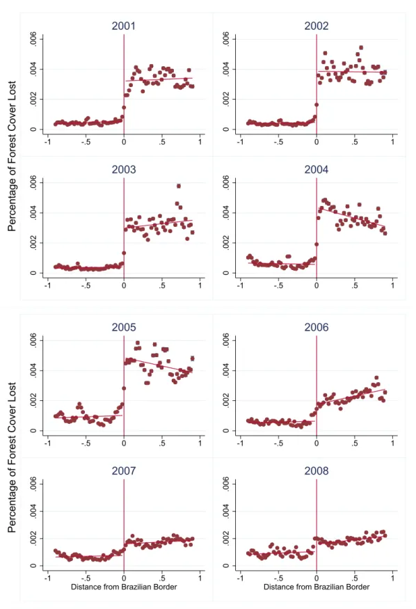
We next plot annual deforestation rates on both sides of the border annually between 2001 and 2014 in Figures 5 and 6. The figures show the percentage of forest cover lost in each year against the distance from the Brazilian border, up to one hundred kilometers from each side of the border. Until 2005, annual forest loss was three to eight times larger on the Brazilian side of the border than on the other side. Annual deforestation rate near the border ranged from 0.3 to 0.4 percent in Brazil, while it ranged from 0.05 to 0.1 percent in the other Amazonian countries. These results point to large differences in national policies which affect deforestation.
Figures 5 and 6 also show us that this dramatic difference in deforestation rates comes to an abrupt halt in 2006. Between 2006 and 2012, deforestation activity is smoothly spread on both sides of the Brazilian border. Although the Action Plan (PPCDAm) was released in 2004, its actions were implemented gradually and we see in Figure 5 that 2006 is a turning point as regards slowing deforestation at Brazil’s borders which often represent the more remote parts of the Amazon.
In particular, 2006 is exactly the year when Brazil promulgates the Law on Public Forest Management, when IBAMA’s Center for Environmental Monitoring (CEMAN) became fully operational and when the local operational basis from IBAMA started re-ceiving online deforestation data (MMA, 2008). In 2013 and 2014, deforestation on the Brazilian side starts to increase, but if we attend to the scale of the graphs we see that the deforestation activity around the border in 2014 is similar to 2006’s one, and still substan-tially smaller than pre-Action Plan levels. This apparent trend reversal may be credited to large infrastructure projects being built in the Amazon area, or the New Forestry Code approved in 2012 which gave greater flexibility to agricultural land use and decentralized operational activities to the States (Ferreira et al., 2014).
The estimates of our spatial discontinuity regression (1) corroborate the graphical evidence. Table 3, columns 2-15, present the estimates of the Brazilian institutions effect, γ, by annual forest loss from 2001 and 2014. Figure 7 presents the point estimates using a 17 km bandwidth shown in Table 3 Panel A, with the vertical bars representing 95% confidence intervals. We see that in each year until 2005 the probability that a forested pixel was deforested on the Brazilian side of the border was around four times the rate on the other side of the border – see Table 1 for the summary statistics. In 2004, for example, the probability that a given forest plot was deforested near the border outside
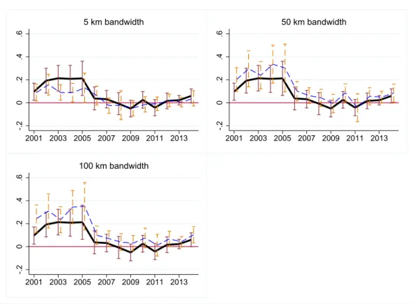
Brazil was around 0.083 percent whilst the deforestation rate on the Brazil side of the border was 0.422 percent. This difference is statistically significant at 1 percent. Point estimates are increasing with the bandwidth but remain substantial in magnitude and statistically significant even using just those pixels within 5 km of the border, as can be seen in Figure 8.
We therefore are finding that the national policies and institutions do matter at the border, both for level of deforestation in 2000 and for subsequent deforestation rates until 2005. However, we see that coincidentally with the Action Plan (PPCDAm), from 2006 onwards, this new raft of Brazilian policies eliminate the differential in deforestation rates between Brazil and her neighbors. Figure 7 and Table 3 (columns 7-15) shows that our estimates of the effect of Brazilian institutions at the border, γ, become smaller and not statistically significant. For some years, the point estimates considering larger bandwidths – Panels C and D – are statistically significant, but these are at least a third of the point estimates for 2004.
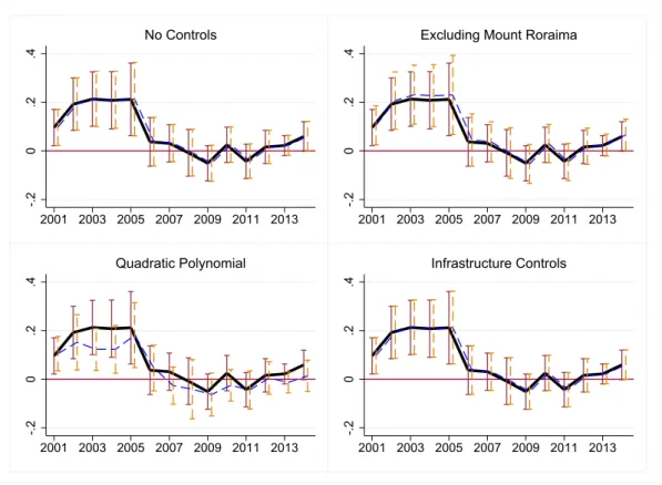
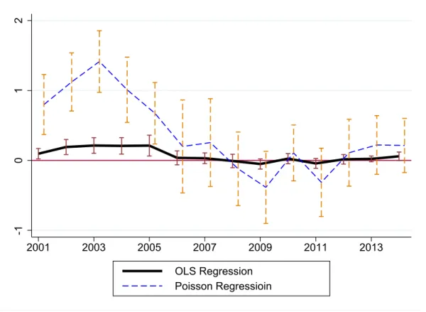
These results are robust to a series of alternatives specifications and samples, using the 17 km bandwidth, as shown in Figure 9 and in Table 4. Panel A presents results when we do not controls for the slope of the terrain and distance to water and use only linear polynomials of distance to the border as controls. Panel B excludes a 220km buffer around the peak of Mount Roraima, a small section of the northern border with Venezuela, which is coincident with a mountain ridge. Panel C uses quadratic polynomials of distance to the border as control. Panel D adds four infrastructure controls: the distance to roads, the distance to Brazilian roads, the distance from urban areas and the distance from Brazilian urban areas. In all these specifications, the estimated results are very close to the ones presented in Table 3 Panel A. The results are also robust when we estimate using a Poisson regression, as can be seen in In Figure 10 and in Table 4 Panel F.
In Figure 11 and in Table 4 Panel E, we estimate the effect of Brazilian institutions restricting the sample to areas around artificial borders as in Alesina et al. (2011) – i.e. those which are literally straight lines drawn on a map, as opposed to following natural features such as rivers.21 For these borders, there is no geographic feature at the border – and indeed, usually not even so much as a fence. Nevertheless, we find even larger effects: a 10 percentage point difference in deforestation at artificial borders in 2000, and around 0.5 percentage point difference in annual forest loss in 2003 and 2004.
4.2
Heterogeneity
Our results point that Brazilian institutions matter overall. We now document evidence of heterogeneity in institutions across different segments of the border and different land
types within Brazil. We first investigate heterogeneous results across different country borders. We examine the Brazilian borders with Bolivia, Peru, Columbia, Venezuela, Guyana, Suriname, and French Guyana.22 We observe substantial differences in baseline magnitudes of deforestation in different parts of Amazon, with the highest deforestation in the “Arc of Deforestation” where the Amazon frontier intersects the border with Bolivia and Peru.23 To deal with this, in this section we present estimate equation (1) using Poisson regressions so results are consistently interpretable as relative increase in the Brazilian side.
Results for the different border segments are shown in Figures 12 and 13 and in Tables 5 and 6. We can see that in all fourteen years for which we have data available, Brazilian national policies have largely no effect on deforestation pattern near the Brazilian border with four of these countries. We can see that the main differences in deforestation rates are found around the border with Bolivia and Peru, around the “ Arc of Deforestation”. We also find a meaningful difference in deforestation rate at the border with Suriname, but this represent a smaller area and the estimates are noisier. The estimates presented in Figure 12 suggest that, until 2005, Brazilian national policies affected deforestation rate around the border with Bolivia are comparable with the the national average.24
The fact that we find differential deforestation concentrated around the border with Bolivia and Peru could have two reasons: Bolivian and Peruvian policies could be partic-ularly good to cope with deforestation, or local policies within Brazil could be particpartic-ularly problematic in that region. Evidence suggest that it is the latter. First, as shown in Table A1 and Figure A1 in the appendix, the Bolivian Amazon had the smallest share of Ama-zon forest cover in 2000 and second highest deforestation rates in the following fourteen years, just behind Brazil. Although Peru had high forest cover in 2000, the country had the third highest deforestation rate between 2001 and 2014. That is, compared with all other countries in the Amazon area, Bolivia and Peru does not seem to be particularly effective in deterring deforestation. Second, as we argue above, the area within Brazil near the border with Bolivia is at the forefront of deforestation, this is an area pressed in between the national frontier and the large-scale agricultural frontier.
We also investigate heterogeneity in policies within the Brazilian side. We find evi-dence that Brazilian laws and its enforcement, as well the changes brought by the Action Plan, and not particularly good Bolivian or Peruvian policies, were responsible for the dif-ferential policies effects estimated at the border. As we describe in section 2.1.3, although most deforestation is illegal in Brazil, certain areas have special legal protections and other areas gained additional legal protection with the PPCDAm. Until 2005, destroying
22Table A1 in the appendix show the area of Amazon in each country, as well as key summary statistics. 23The “Arc of Deforestation” is the area where the forest is more under pressure from urbanization
and the expansion of the agriculture frontier in the Midwest of the country.
or harming native vegetation in Protected Areas was a crime subject to harsher legal pro-cedures and punishments – including possible jail time – than deforesting vegetation in non-protected areas. Also, Protected Areas are cannot have large scale cash crops under severe legal consequences for the land owner. We see in Figure 14 and in Table 7 Panel A that when the national border abuts these protected areas there is less deforestation on the Brazilian side in all period studied. This suggests that areas with initial stronger land regulation in Brazil actually contributed to keep deforestation rate low.
However, as Figure 14 and Table 7 Panel B show, when the national border does not abut a protected area there is more deforestation on the Brazilian side, at least until 2005. In that year, PPCDAm changed the regulation and punishment for deforesting non-protected areas: it increased the minimum set aside area of private rural properties from 35% to 80%, and turned deforestation of unclaimed lands into a felony, thereby, increasing its potential punishment. Since the legal consequences for deforesting protected areas stayed unchanged, we would expect that these legal changes would affect local policies only in non-protected areas. Evidence corroborate this intuition. We find no meaningful change on the Brazilian policies in these protected areas – land already with more stringent environmental regulation – in the whole period studied. The estimates in Panel B of this same table show that local policies in non-protected areas led to annual deforestation rates around 0.5 percentage points higher on the Brazilian side of the border until 2005, and these effects dropped sharply in 2006 onwards by around one third relative pre-PPCDAm, often imprecisely estimated. This shows that the national policies effect is not being driven by the fact that deforestation is uniformly more profitable in Brazil, but rather by different legal and enforcement regimes within Brazil.
We document further evidence of heterogeneity in the local implementation of the national policies within the Brazilian side. As part of the Action Plan (PPCDAm), the government black listed more than 50 counties due to high deforestation activities in the Amazon. Only two black listed counties are at the Brazilian border; and both share a border with Bolivia – these are Nova Mamoré and Porto Velho. Figure 16 and Table 8 Panels A and B present our results when we split the sample in border segments on black listed counties and counties not black listed. We see that Brazilian institutional effect on forest cover in 2000 is around one order of magnitude higher in black listed counties than in counties not black listed; local policies in black listed counties led to 22 percentage points less forest cover in 2000, as compared to only 2.7 percentage points in all other counties at the border. That is, in terms of deforestation these are areas with particularly bad local institutions within Brazil. This analysis shows that the areas singled out for the black list are not having higher deforestation because of higher local demand factors; it really appears to be worse governance, since the effects on deforestation are largely limited to the Brazilian side of the border.
Table 8 Panel A and B – columns 2 to 6 – also show that, until 2005, Brazilian policies led to higher deforestation rate on average in both black listed and non-black listed counties, however the effects were between two to six times higher for black listed counties. We can see in Panel B – columns 7 to 15 – that the differential rate in annual forest loss in Brazil relative other countries disappear from 2006 onwards in non-black listed counties, as discussed before. Importantly, we do not observe a meaningful reduction in the large impacts on deforestation of local policies in black listed counties. Brazilian local policies in these areas continued leading to higher annual deforestation until 2013. This suggests that local institutions could pose limits to the reach of national policies.25
Clearly, access to infrastructure, such as roads, matters for deforestation (Pfaff, 1999) and could as well impose limits to the reach of the state. We investigate heterogeneity according to proximity to roads by splitting our sample in pixels on either side of the border that are within 5 km of a road, or pixels that are more than 5 km away from the nearest road. In fact, Table 8 Panels C and D show that all differential effect of national policies at the baseline forest cover comes from pixels close to roads; by contrast, when we examine pixels more than 5 km away from a road on either side of the border we find largely no difference on baseline forest level. However, until 2005, we find proportionally higherannual deforestation rate on the Brazilian side for pixels near to and distant from road network. Figure 17 and Table 8 Panels C and D present these estimates. We find that the higher deforestation rate on the Brazilian side reverted faster in pixels near roads, while the decline in forest loss in pixels more distant from roads started only three years later. This suggests that proximity to roads – or infrastructure – is necessary for intense deforestation to take place and for national policies to reach, but it is not sufficient. National and local policies are important to deforestation on top of the existence of basic infrastructure, and can be shaped to help coping with deforestation.
4.3
Quantifying the magnitude of the border effect
Proximity to roads are important for deforestation, but other characteristics of the land may also affect the propensity that each plot of forest will be cut down. For example, proximity to urban areas, proximity to rivers and the slope of the terrain also influence the cost of deforesting a given plot of land or may affect the expected productivity of that plot. Pixels’ geographic characteristics provide us some information about the expected profitability of converting each forested plot of land into other use. To quantify the magnitude of the border effects, we use a logit model to estimate the probability that each pixel is deforested in 2001 as a function of observable factors. We restrict our sample to Brazilian land up to 17 km from the border with Bolivia, the area with higher
25Adman (2014) investigates the mechanisms within black listed counties that acted to reduce
deforestation activity in Brazil. We include the following pixels’ characteristics in our estimation: the level and the squared values of slope, distance to water, distance to roads and distance to urban areas. We use the parameters estimated using forest loss in 2001 in Brazilian territory (see Appendix Table A2) to predict the propensity that each pixel in Bolivia is deforested based on their characteristics.
This allows us to quantify the Brazil effect in terms of observables as we compare the propensity of being deforested of pixels that were actually deforested in Brazil and in Bolivia. Figure 18 present the predicted probability that each pixel would be deforested for all pixels actually deforested each year in Brazil (solid red line) and in Bolivia (blue dashed line). We see that, until 2005, pixels deforested on the Brazilian side of the border had on average a smaller propensity to be deforested based on their observable characteristics than the pixels that were deforested on the Bolivian side of the border. In other words, in a period when a much larger area was being deforested on the Brazilian side of the border, pixels deforested in Bolivia tended to be around 25 percent more profitable than those deforested in Brazil if we considered only their geographic characteristics. That is, it must be that unobservable factors of the Brazilian pixels, such as land regulation and policies, where underlying the higher deforestation rate on the Brazilian side. Interestingly, this gap starts to revert after 2005, when the pixels with higher propensity to deforest in Bolivia start to be deforested – potentially low ranging fruits. This is exactly when the border effect estimated in Table A8 Panel A become statistically equal to zero. By the end of the period, the average propensity to deforest of deforested pixels in Brazil and Bolivia become level.
4.4
Results for DR Congo and Indonesia
We now take the Brazilian case as a benchmark and investigate if a deterioration of national policies may explain the upward deforestation trends observed in DR Congo and Indonesia as we discussed in the introduction. Figures A6 and B and Table A13 in the Appendix C present the results for DR Congo. Although we cannot clearly see in Figure A6, the point estimates in Table A13 suggest that there was discontinuously higher forest cover in 2000 in DRC than in its bordering countries. In Figure B, we see no differential annual forest loss in the border except in 2010, when we observe a sharp break on the estimated effects in deforestation rate which reverts fast over the following two years. Looking closer at the data and satellite images, this seems to be a localized effect actually due to a fast increase in deforestation in Zambia just by the border.
Figures A8 and B and Table A13 in the Appendix D present the results for the South-ern Indonesia and Papua New Guinea border. We find no robust differential deforestation activity at the border, both in levels in 2000 and subsequent annual forest loss.
in DRC and Indonesia do not seem to be due to a deterioration of national deforestation policies. However, the absence of strong national environmental policies likely disabled these countries to counteract the increasing local and market pressure that led to increas-ing forest losses in the period.
5
Conclusion
We estimate spatial regression discontinuity designs at the national border between Brazil and surrounding countries to identify the effect of national institutions deep in the hinter-land. Our results show that national institutions and policies are important at the border: both baseline forest cover and annual deforestation rate change abruptly at the border – we find higher deforestation activity on the Brazilian side of the border. Furthermore, we find evidence of heterogeneous institutions within Brazil – the bulk of deforestation happened in forest areas subject to weaker and more lenient laws – non-Protected Areas. We also document that weak institutions can be strengthen in a short period of time. Following the Brazilian government released a action plan for prevention and control of deforestation in the Amazon (PPCDAm) – which enacted a harsher legal framework against deforestation in non-protected areas – we estimate that negative effect of Brazilian institutions at the border virtually disappear from 2006 onwards. We find that the bulk of this change happened in areas near roads, where access was substantial, and within non-protected areas, exactly the areas that were subject to the legal changes. The results demonstrate the power of concerted state enforcement even in the deep hinterlands.
References
Adman, Ryan. 2014. Reelection Incentives, Blacklisting and Deforestation in the Brazil-ian Amazon. Tech. rept. .
Alesina, Alberto, Easterly, William, & Matuszeski, Janina. 2011. Artificial states. Journal of the European Economic Association, 9(2), 246–277.
Alston, Lee J, Harris, Edwyna, & Mueller, Bernardo. 2012. The development of property rights on frontiers: Endowments, norms, and politics. The Journal of Economic History, 72, 741–770.
Assunção, Juliano, Gandour, Clarissa, & Rocha, Romero. 2013a. DETERring Deforestation in the Brazilian Amazon: Environmental Monitoring and Law Enforce-ment. Tech. rept. Climate Policy Institute.
Assunção, Juliano, Gandour, Clarissa, Rocha, Romero, & Rocha, Rudi. 2013b. Does Credit Affect Deforestation? Evidence from a Rural Credit Policy in the Brazilian Amazon. Tech. rept. Climate Policy Institute.
Assunção, Juliano, Gandour, Clarissa C, & Rocha, Rudi. 2015. Deforestation slowdown in the Legal Amazon: prices or policies? Environment and Development Economics, 20(6), 697–722.
Barber, Christopher P, Cochrane, Mark A, Souza, Carlos M, & Laurance, William F. 2014. Roads, deforestation, and the mitigating effect of protected areas in the Amazon. Biological conservation, 177, 203–209.
Burgess, Robin, Hansen, Matthew, Olken, Benjamin A, Potapov, Peter, Sieber, Stefanie, et al. 2012. The Political Economy of Deforestation in the Tropics. The Quarterly Journal of Economics, 127(4), 1707–1754.
Cardoso, Fernando Henrique, & Winter, Brian. 2007. The accidental president of Brazil: a memoir. PublicAffairs.
Conley, Timothy G. 1999. GMM estimation with cross sectional dependence. Journal of Econometrics, 92, 1–45.
D’Anville, Jean-Baptiste Bourguignon. 1779 (Aout 10). Mémoire sur un accoisse-ment considérable de connoissances locales en ce qui intéresse l’Amérique méridionale. Robert Bosch Collection, Stuttgart, Germany. n. 539, 11p.
Ferreira, J., Aragão, L. E. O. C., Barlow, J., Barreto, P., Berenguer, E., Bustamante, M., Gardner, T. A., Lees, A. C., Lima, A., Louzada, J., Pardini, R., Parry, L., Peres, C. A., Pompeu, P. S., Tabarelli, M., & Zuanon, J. 2014. Brazil’s environmental leadership at risk. Science, 346(6210), 706–707.
Furtado, Júnia Ferreira. 2012. Oraculos da geografia ilumisnista: Dom Luís da Cunha e Jean-Baptiste Bourguignon d’Anville na construção da cartografia do Brasil. Editora UFMG.
Gelman, Andrew, & Imbens, Guido. 2014. Why high-order polynomials should not be used in regression discontinuity designs. Tech. rept. National Bureau of Economic Research.
Godar, Javier, Gardner, Toby A, Tizado, E Jorge, & Pacheco, Pablo. 2014. Actor-specific contributions to the deforestation slowdown in the Brazilian Amazon. Proceedings of the National Academy of Sciences, 111, 15591–15596.
Hansen, Matthew C, Potapov, Peter V, Moore, Rebecca, Hancher, Matt, Turubanova, SA, Tyukavina, Alexandra, Thau, David, Stehman, SV, Goetz, SJ, Loveland, TR, et al. 2013. High-resolution global maps of 21st-century forest cover change. Science, 342, 850–853.
Hargrave, Jorge, & Kis-Katos, Krisztina. 2013. Economic causes of deforestation in the Brazilian Amazon: a panel data analysis for the 2000s. Environmental and Resource Economics, 54, 471–494.
Herbst, Jeffrey. 2000. States and Power in Africa: Comparative Lessons in Authority and Control. Princeton University Press.
Holmes, Thomas J. 1998. The effect of state policies on the location of manufacturing: Evidence from state borders. Journal of Political Economy, 106(4), 667–705.
Imbens, Guido, & Kalyanaraman, Karthik. 2012. Optimal bandwidth choice for the regression discontinuity estimator. The Review of Economic Studies, 79, 933–959. Michalopoulos, Stelios, & Papaioannou, Elias. 2014. National Institutions and Subnational Development in Africa. The Quarterly Journal of Economics, 129(1), 151–213.
MMA, Ministério do Meio Ambiente. 2008. Plano de Ação para Prevenção e Cont-role do Desmatamento na Amazônia Legal (PPCDAm). Documento de Avaliação 2004-2007.
MMA, Ministério do Meio Ambiente. 2013. Plano de Ação para Prevenção e Con-trole do Desmatamento na Amazônia Legal (PPCDAm) 3a Fase (2012-2015) pelo uso sustentável e conservação da Floresta. Brasília.
Nepstad, Daniel, Soares-Filho, Britaldo S, Merry, Frank, Lima, André, Moutinho, Paulo, Carter, John, Bowman, Maria, Cattaneo, Andrea, Ro-drigues, Hermann, Schwartzman, Stephan, et al. 2009. The end of deforestation in the Brazilian Amazon. Science, 326, 1350–1351.
Nepstad, Daniel C, Stickler, Claudia M, & Almeida, Oriana T. 2006. Glob-alization of the Amazon soy and beef industries: opportunities for conservation. Con-servation Biology, 20(6), 1595–1603.
Nolte, Christoph, Agrawal, Arun, Silvius, Kirsten M, & Soares-Filho, Britaldo S. 2013. Governance regime and location influence avoided deforestation suc-cess of protected areas in the Brazilian Amazon. Proceedings of the National Academy of Sciences, 110(13), 4956–4961.
Pfaff, Alexander SP. 1999. What drives deforestation in the Brazilian Amazon?: evidence from satellite and socioeconomic data. Journal of Environmental Economics and Management, 37, 26–43.
Raza, Salvador. 2013. Brazil’s Border Security Systems Initiative: A Transformative Endeavor in Force Design. Security and Defense Studies Review, 14.
Souza-Rodrigues, Eduardo. 2015. Deforestation in the Amazon: A Unified Frame-work for Estimation and Policy Analysis. Tech. rept. University of Toronto.
0 .2 .4 .6 .8 1 1.2 1.4
Annual Forest Loss
2000 2005 2010 2015
year
Brazil Indonesia DR Congo
Figure 1: Forest Change, 2001-2014, by Country
This figure shows the annual forest loss in Brazil as a whole (including non-Amazon areas), in the Democratic Republic of the Congo and Indonesia. Forest loss is measured as the share of forest cover in each country that was lost in each year – that is, the share of the share of forest cover in year t − 1 that was lost in year t.
.1 .2 .3 .4 .5 .6
Annual Forest Loss (%)
2001 2003 2005 2007 2009 2011 2013 year
Brazil Abroad
Amazon (RAISG limits)
Figure 2: Forest Change, 2001-2014, in the Amazon Area
This figure shows the annual forest loss in the Amazon each year between 2001 and 2014 in Brazil (red line) and other countries (red dashed line). We use the Amazon limits provided by RAISG. Forest loss is measured as the share of forest cover in each country that was lost in each year – that is, the share of the share of forest cover in year t − 1 that was lost in year t.
Figure 3: Example Google Earth Photo of a Border Segment (Percentage of Forest Cover in 2000)
This figure shows the percentage of forest cover in 2000 by 30 meter pixels of a segment of the border between Brazil (North of the border) and Bolivia and Peru (South of the border).
82 84 86 88 90 92
Percentage of Forest Cover in 2000
-1 -.5 0 .5 1
Distance from Brazilian Border (in 100 km)
Figure 4: Average Forest Cover in 2000 by Distance from Brazilian Border
This figure shows the average forest cover in 2000 by 80 equal-sized bins of distances from the Brazilian border, up to 100 kilometers away from the border. Positive distance represent Brazilian land, while negative distance represent non-Brazilian land. The vertical bars (not always visible) depict 95% confidence intervals of the local average within each bin. The red line shows the linear function of distance weighted by the number of observations in each bin.
0 .002 .004 .006 -1 -.5 0 .5 1 2001 0 .002 .004 .006 -1 -.5 0 .5 1 2002 0 .002 .004 .006 -1 -.5 0 .5 1 2003 0 .002 .004 .006 -1 -.5 0 .5 1 2004
Percentage of Forest Cover Lost
0 .002 .004 .006 -1 -.5 0 .5 1 2005 0 .002 .004 .006 -1 -.5 0 .5 1 2006 0 .002 .004 .006 -1 -.5 0 .5 1
Distance from Brazilian Border
2007 0 .002 .004 .006 -1 -.5 0 .5 1
Distance from Brazilian Border
2008
Percentage of Forest Cover Lost
Figure 5: Average Annual Forest Loss at the Border by Year – 2001-2008
This figure shows the average annual forest cover lost each year between 2001 and 2008 by 80 equal-sized bins of distances from the Brazilian border. Each figure present pixels more distant from the border, up 1 hundred kilometers away from the border. Positive distance represent Brazilian land, while negative distance represent non-Brazilian land. The vertical bars (not always visible) depict 95% confidence intervals of the local average within each bin. The red line shows the linear function of distance weighted by the number of observations in each bin.
0 .002 .004 .006 -1 -.5 0 .5 1
2009
0 .002 .004 .006 -1 -.5 0 .5 12010
0 .002 .004 .006 -1 -.5 0 .5 12011
0 .002 .004 .006 -1 -.5 0 .5 12012
0 .002 .004 .006 -1 -.5 0 .5 1 Distance from Brazilian Border2013
0 .002 .004 .006 -1 -.5 0 .5 1 Distance from Brazilian Border2014
Percentage of Forest Cover Lost
-.1 0 .1 .2 .3 .4 2001 2003 2005 2007 2009 2011 2013 year
Figure 7: Regression Discontinuity Coefficients by Year – Main Specification This figure shows the regression discontinuity coefficients of the Brazilian effect, γ, on the percentage of annual forest loss by year, from equation (1) with linear polynomials and 17 km bandwidth, as shown in Panel A Table 3. The vertical bars represent 95% confidence intervals.
-.2 0 .2 .4 .6 2001 2003 2005 2007 2009 2011 2013 5 km bandwidth -.2 0 .2 .4 .6 2001 2003 2005 2007 2009 2011 2013 50 km bandwidth -.2 0 .2 .4 .6 2001 2003 2005 2007 2009 2011 2013 100 km bandwidth
Figure 8: Regression Discontinuity Coefficients by Year – Different Bandwidth This figure shows the regression discontinuity coefficients of the Brazilian effect, γ, on the percentage of annual forest loss by year, from equation (1) with linear polynomials and 17 km bandwidth, as shown in Panels B to D Table 3. The vertical bars represent 95% confidence intervals.