Nhan Phan
Developing Robo-advisor Software with Semivariance and Black-Litter- man Model
Metropolia University of Applied Sciences Bachelor of Engineering
Degree Programme in Information Technology Bachelor’s Thesis
15 May 2020
Author Title
Number of Pages Date
Nhan Phan
Developing robo-advisor software with semivariance and Black- Litterman model
37 pages + 1 appendix 15 May 2020
Degree Bachelor of Engineering
Degree Programme Information Technology Professional Major Smart Systems
Instructors
Sami Sainio, Senior Lecturer
The purpose of this thesis was to develop a robo-advisor program for Japanese pension investment fund. A robo-advisor can reduce behavioral biases and provide an objective sug- gestion for investors. The program will make an investment recommendation on bond and stock market of major economies in North America, Europe and Asia.
The program is based on Markowitz’s Modern Portfolio Theory. The Markowitz framework is used to compute optimal investment portfolios that offer the highest level of expected return for a predetermined level of risk. However, since its release in 1952, many and even Markowitz himself have suggested improvements to the model to improve its application in real world problems. Therefore, the program also implements semivariance, Black-Litterman model and portfolio simplification into the traditional model.
Due to the large amount of data and the complexity of the program, the program must be capable of computing convex optimization with reasonable speed. Program development also takes into consideration the broad user group. To make sure anyone without technical skill can use the model, the program was designed to target simplicity and usability.
Python with CVXPY library for convex optimization and Tkinter for GUI library were chosen for program development. Other Python libraries, NumPy and pandas, were deliberately used due to their ability in handling data and solve mathematic equations.
Improvements were backtested using 10 years of ETF historical data from Bloomberg. The results showed that those improvements reduce the limitation of Modern Portfolio in real world and generally raise the return of the investment. However, further studies should be considered during the extreme market condition.
Based on the backtest result, the final program is a useful tool for asset allocation. However, its limitation in using historical return to forecast is not fully eliminated. Further implementa- tion will focus on developing a better return prediction model, based on the asset’s potential and not on its past performance.
Keywords portfolio optimization, cvxpy, semivariance, Black-Litterman
Contents
List of Abbreviations
1 Overview 1
2 Modern Portfolio Theory 2
2.1 Return and risk 2
2.2 Efficient Frontier 4
2.3 Sharpe Portfolio and Minimum Variance Portfolio 6
2.4 Criticisms 6
2.5 Black-Litterman model 7
3 Implementation 9
3.1 Programming Language and Libraries 9
3.2 Portfolio Construction 12
3.2.1 Equity construction 12
3.2.2 Bond and Alternative Investment Construction 15
3.3 Program flowchart 16
3.4 Program user interface 19
4 Improvement 23
4.1 Semivariance 24
4.2 Black-Litterman model 27
4.3 Portfolio Simplification 30
5 Conclusion 33
5.1 Summary 33
5.2 Discussion 34
References 36
Appendix
Appendix 1. Portfolio allocation in March 2020
AUM Assets under management. The total market value of all the financial as- sets which a financial institution manages on behalf of its client and them- selves.
STDEV Standard deviation. Statistics number measures the variation of a data set within a period.
EF Efficient Frontier
ETF Exchange-traded fund. It’s a type of security that often tracks an underlying index and is listed on stock exchange. ETF can be traded on stock ex- change like a normal stock.
GDP Gross domestic product
BL Black-Litterman. Black-Litterman model is a financial model in portfolio al- location.
GUI Graphical user interface
1 Overview
According to U.S Securities and Exchange Commission, robo-advisors are automated digital investment advisory programs, which provide investment advice with minimum human interaction [1]. Customer enters their financial information into those programs and receives investment service, with potential benefit of lower managing costs com- pared with traditional services. In the 1st quarter of 2018, Backend Benchmarking esti- mated the total assets under management (AUM) of those robo-advisors is close to $178 billion [2]. Two years later, in their 4th quarter of 2019 report, Backend Benchmarking approximate total AUM have increased 50% to $275 billion [3]. The main hypothesis of this thesis is that by developing a robot investment software based on the improved Mar- kowitz’s Modern Portfolio Theory, it builds a solid theoretical foundation for the model and subsequently is possible to improve the return of investment compared to existing robo-advisors.
Other renown investment banks, such as Goldman Sachs or JPMorgan Chase, are in- vesting in quantum computing technology. A quantum computer can solve complex Monte Carlo simulations fast and can provide portfolio optimization service for bank’s clients. However, experts believe there are a lot of challenges and expect it would take them at least 5 years to achieve the desirable outcome [4]. Even with the algorithm and hardware for quantum computing would be available, the availability of such quantum computers will be limited. The program developed in this thesis will still benefit the regular stock market investors.
Without quantum technology breakthrough, we can challenge this problem with a simpler solution, by building an investment advisor program based on a famous economic theory:
Modern Portfolio Theory. Modern Portfolio Theory allow us to construct a line of optimal portfolios – Efficient Frontier (EF) – that can dynamically change with new information.
The theory was first introduced by Harry Max Markowitz in 1952 and brought him the 1990 Nobel Memorial Prize in Economic Sciences [5].
2 Modern Portfolio Theory
2.1 Return and risk
Asset return is the historical return of asset within a period, often longer than one year.
In practical, and in this thesis, asset return is calculated yearly unless stated otherwise.
Because we average asset return using geometric method instead of arithmetic method, asset return is also called compound annual growth rate (CAGR). For example, if price of stock A was $100 in 31/12/2015, and was $150 in 31/12/2018. Stock A’s CAGR and yearly return is √150
100
3 − 1 = √1.53 − 1 = 14.47% (a year).
Asset risks are measured using standard deviation (STDEV). In statistics, STDEV was used to measure the variety of a data set within a period. In finance, investors use STDEV to measure the volatility of their investment return [6, p. 182]. Assets with high STDEV have high uncertainty that their actual return will be the same as their expected return and therefore investors regard them as high-risk asset.
Portfolio return, or expected return is calculated by taking the sum of the product of indi- vidual asset return in the portfolio with the weight of that asset in the portfolio. As asset return is CAGR, portfolio is also CAGR. Formula to calculate portfolio return is:
𝑃𝑜𝑟𝑡𝑓𝑜𝑙𝑖𝑜 𝑟𝑒𝑡𝑢𝑟𝑛 = ∑𝑛𝑖=1𝑤𝑖× 𝑟𝑖 (1)
where 𝑤𝑖 is weight of asset 𝑖 in portfolio, and 𝑟𝑖 is return of asset 𝑖.
Portfolio risk is more complex than other parameters. On one hand, it has the same interpretation of asset risk, as it also measured risks using standard deviation. On the other hand, it requires more input parameters than portfolio return, and the number of input parameter increases aggressively the more asset we include in our portfolio. Com- parable to portfolio return, portfolio risk requires asset return and asset weight. It, how- ever, requires the third parameter: correlation between two different assets in the portfo- lio. If our portfolio only consists of asset A and asset B, we only need to compute
correlation between asset A and asset B. When include asset C in our portfolio, we will need to compute correlation between A and B, B and C, and finally A and C
𝜎𝐴𝐵2 = 𝑤𝐴2𝜎𝐴2+ 𝑤𝐵2𝜎𝐵2+ 2𝑤𝐴𝑤𝐵𝜎𝐴𝜎𝐵𝜌𝐴𝐵
𝜎𝐴𝐵𝐶2 = 𝑤𝐴2𝜎𝐴2+ 𝑤𝐵2𝜎𝐵2 + 𝑤𝐶2𝜎𝐶2+ 2𝑤𝐴𝑤𝐵𝜎𝐴𝜎𝐵𝜌𝐴𝐵+ 2𝑤𝐴𝑤𝐶𝜎𝐴𝜎𝐶𝜌𝐴𝐶+ 2𝑤𝐵𝑤𝐶𝜎𝐵𝜎𝐶𝜌𝐵𝐶
In general, the portfolio variance (𝜎𝑝2) is calculated by the formula
𝜎𝑝2= ∑ 𝑤𝑖 𝑖2𝜎𝑖2+ ∑ ∑𝑖 𝑗≠𝑖𝑤𝑖𝑤𝑗𝜎𝑖𝜎𝑗𝜌𝑖𝑗 (2)
where 𝜎𝑖 is STDEV of asset 𝑖 in portfolio, 𝑤𝑖 is weight of asset 𝑖 in portfolio, 𝜌𝑖𝑗 is corre- lation between asset 𝑖 and asset 𝑗.
Using the formula (2) in programming would require loop functions to get all possible companions of two assets to calculate portfolio risk. Instead, we can use matrix and vector for variance, and for more complex model introduced in next section. To be able to use matrix to calculate variance, first we need to calculate covariance, which measure the combined movement of returns on two assets. Like variance, covariance measures the volatility of return, but between two assets. Covariance can be calculated from as- sets’ STDEV and their correlation by using formula:
𝐶𝑜𝑣𝑖,𝑗= 𝜌𝑖𝑗𝜎𝑖𝜎𝑗 (3)
From the formula above, we can see that covariance between two assets that have no correlation which other is 0, and covariance between asset 𝑖 and itself is its variance. We can calculate covariance matrix of a portfolio P with 𝑚 assets by using matrix multiplica- tion:
[
𝐶𝑜𝑣11 ⋯ 𝐶𝑜𝑣1𝑚
⋮ ⋱ ⋮
𝐶𝑜𝑣𝑚1 ⋯ 𝐶𝑜𝑣𝑚𝑚 ] = [
𝜎1 ⋯ 0
⋮ ⋱ ⋮
0 ⋯ 𝜎𝑚 ] × [
𝜌11 ⋯ 𝜌1𝑚
⋮ ⋱ ⋮
𝜌𝑚1 ⋯ 𝜌𝑚𝑚] × [
𝜎1 ⋯ 0
⋮ ⋱ ⋮
0 ⋯ 𝜎𝑚
] (4)
where [
𝜎1 ⋯ 0
⋮ ⋱ ⋮
0 ⋯ 𝜎𝑚
] is the diagonal matrix (all values outside the main diagonal are zero)
of assets’ STDEV, and [
𝜌11 ⋯ 𝜌1𝑚
⋮ ⋱ ⋮
𝜌𝑚1 ⋯ 𝜌𝑚𝑚] is correlation matrix of all 𝑚 asset in portfolio.
After getting covariance matrix, we can calculate the portfolio variance:
𝜎𝑝2= [ 𝑤1
⋮ 𝑤𝑚]
𝑇
× [
𝐶𝑜𝑣11 ⋯ 𝐶𝑜𝑣1𝑚
⋮ ⋱ ⋮
𝐶𝑜𝑣𝑚1 ⋯ 𝐶𝑜𝑣𝑚𝑚 ] × [
𝑤1
⋮
𝑤𝑚] (5)
where [ 𝑤1
⋮
𝑤𝑚] is weight vector of all assets in portfolio
2.2 Efficient Frontier
Efficient Frontier (EF) is a curve line contains all the best portfolios possible from a com- bination of assets. Its x-axis represents the risk (STDEV or variance) of the portfolio, while its y-axis represents the expected return. When first introduced by Markowitz, it was called the Efficient E, V (Expected Return, Variance) Combinations [7]. The graph of an EF is shown in Figure 1 below. The following exchanged-traded fund (ETF) were used with 5 years monthly data to construct the EF at the end of 31 March 2020: SPY (SPDR S&P 500 ETF Trust), EMB (iShares JP Morgan USD Emerging Markets Bond), BIV (Vanguard Intermediate-Term Bond ETF), IWF (iShares Russell 1000 Growth ETF), VIG (Vanguard Dividend Appreciation ETF), XLK (Technology Select Sector SPDR Fund). The EF was built using the robo-advisor software, while randomized portfolios were obtained by randomized the weight of each ETF in the portfolio. While the EF is much longer, since the Sharpe Portfolio and Minimum Variance Portfolio were the focus, the rest of the EF line was cut out.
Figure 1. The Efficient Frontier
As illustrated in Figure 1, any point below the EF is a worse investment, as it offers lower expected return for the same amount of risk. Any rational and risk averse investor will not pick suboptimal portfolio, as it is an assumption in the Modern Portfolio Theory. It is also impossible to find any point higher than the EF, because the EF already contain all the highest possible expected return with a predetermined level of risk. Also note that the lower half of the EF (the line below 4.74% expected return) is not efficient, as we can replace it with any point in the upper half and have higher return with the same level of risk.
With the EF, investors can invest their money into the market with the expectation that their portfolio offers the highest expected return possible. Investors who want higher ex- pected return can move along the EF line to the right, as it offer higher expected return by taking higher risk.
3.0%
4.0%
5.0%
6.0%
7.0%
8.0%
9.0%
10.0%
11.0%
3.0% 4.0% 5.0% 6.0% 7.0% 8.0%
Portfolio expected return
Portfolio Stdev
Efficient Frontier
Efficient Frontier Randomized Portfolio Sharpe Portfolio Minimum Variance Portfolio
2.3 Sharpe Portfolio and Minimum Variance Portfolio
In Figure 1, there are two important portfolios. The first is Sharpe Portfolio, which have expected return of 7.02% and STDEV of 4.47%. The Sharpe Portfolio, by our own defi- nition in this work, is the portfolio with the highest Sharpe ratio. William F. Sharpe intro- duced the ratio in 1966, and later revised it in 1994 with the name Ex Ante Sharpe Ratio [8]:
𝑆ℎ𝑎𝑟𝑝𝑒 𝑟𝑎𝑡𝑖𝑜 = 𝔼(𝑅𝐹−𝑅𝐵)
𝜎𝐹 (6)
where 𝑅𝐹 is return on portfolio F, 𝑅𝐵 is return on benchmark (risk free rate) and 𝜎𝐹 is STDEV of portfolio F (with B is risk free rate).
Based on the above formula, the Sharpe ratio measure the expected excess return (port- folio return minus risk free rate) per unit of risk. The Sharpe Portfolio in Figure 1 have the highest Sharpe ratio of 1.4841 with risk free rate at 0.3844%, which mean for every unit of risk taken at that point, investor will be expected 1.4841 unit of excess return. As we move long the EF, the further away we get from the Sharpe Portfolio, the lower the Sharpe ratio we get, and lower excess return per each unit of risk we take. As different investors have different risk profiles, we cannot set a predetermined level of risk for our portfolio during our work. Therefore, we will base our thesis on the Sharpe portfolio, and investors will have option to adjust their risk level to suit their need in the final software.
The second important portfolio in Figure 1 is the Minimum Variance Portfolio (expected return: 4.74%, STDEV: 3.49%, Sharpe ratio: 1.25). It is the portfolio on the EF line that have the lowed STDEV among all possible portfolio. This portfolio would be the most suitable one for low risk tolerance investors.
2.4 Criticisms
In Modern Portfolio Theory, return, risk and other related parameters are calculated based on historical data. Therefore, the prediction power of the model is based on his- torical events. However, if there is a new event happen in future that never happened
before, such as the global coronavirus pandemic in 2020, then the model will fail to eval- uate that event. One common warning in finance research report is that past perfor- mance is not a guarantee of future results, and Modern Portfolio Theory is using past performance to calculate portfolio expected return. In their research in 1991, Best and Grauer found that a small change in assets’ expected return will result in a significant change in portfolio allocation [9]. Therefore, any small error in the estimation of expected return will lead to a notable different in investment performance.
Another criticism of Modern Portfolio Theory is that it measures risk in term of volatility.
However, many investors don’t view STDEV as risk. Warren Buffett, a famous and suc- cessful investor, once said that his partner and him would “much rather earn a lumpy 15% over time than a smooth 12%” [10]. For him, and for many investors, volatility is a part of stock investment and should not be a negative point when investing. This can be improved by using semivariance to measure the volatility when stock return is lower than expected instead of variance. We will discuss this in chapter 4.1.
2.5 Black-Litterman model
Among criticisms mentioned in chapter 2.4, using historical data to predict future return is rationally the most important point, as any small error would result in a critical different in the result. To address this problem, Fischer Black and Robert Litterman developed a model, named the Black-Litterman (BL) model. The BL model combine the expected return of a diversified market portfolio with the investor’s subjective view to form a inves- tors’ expected return instead of the traditional expected return in Modern Portfolio Theory [11]. First, the concept of equilibrium expected return, the level of return that adequately compensate investors for their expected risk, was discussed. The BL model assumes that there are equilibrium expected returns in the market. Each asset has their own value of equilibrium expected return. And combine with their equilibrium weight, they form the equilibrium market portfolio that reflect the investors’ expectation of the capital market.
By solving for the implied equilibrium return, and include investors’ view into the model, we get market’s expected return, instead of historical expected return, for our model.
The BL model require several steps to find the investors’ view-adjusted market equilib- rium returns [12]:
• Determine market portfolio and equilibrium market weight. Calculate covariance matrix for all assets. Market portfolio, and subsequently market weight is based on the investors’ investment geography. For example, an investor invest in United States equity only will consider all listed equities in United States as his market portfolio, and all equites weight, determined by their market capitalization, in that portfolio as equilibrium market weight.
• Perform reverse optimization process. From covariance matrix and asset weight back solving to get the equilibrium expected return. The reverse formula with 𝑚 assets in the portfolio is:
Π= [ 𝑟1
⋮ 𝑟𝑚
] = λ × [
𝐶𝑜𝑣11 ⋯ 𝐶𝑜𝑣1𝑚
⋮ ⋱ ⋮
𝐶𝑜𝑣𝑚1 ⋯ 𝐶𝑜𝑣𝑚𝑚 ]×[
𝑤1
⋮ 𝑤𝑚
] (7)
where Π is the Implied Excess Equilibrium Return Vector, λ is the risk aversion coefficient, calculated by the dividing portfolio excess return by portfolio risk
λ = (𝑟𝑝− 𝑟𝑓)
𝜎𝑝2 (8)
• Set view and confidence for each view. Even though this is an important step in BL model, it requires to set the view without knowing the actual result of the mar- ket in future. This is not suitable for back testing process, where the actual results are known, and will be skipped during model improvement.
• Calculate the view-adjusted market equilibrium return.
• Solve the optimization model and obtain the EF.
The BL were tested in practice and showed that it can help mitigates the problem of over sensitive in estimation [12]. Therefore, we added it into our program as an option for investors to choose for their asset allocation decision.
3 Implementation
While EF is easy to use in investment decision, calculating it is more complex in real world. When we find a good return-risk combination from our assets, we need to assure that return-risk combination is the best we could have. The calculation requires a long computing time, as we need to calculate a list of assets with their weight in the portfolio, get our return-risk combination, and then repeat the process until we are confident that our result is optimal.
3.1 Programming Language and Libraries
Initially, we used Monte Carlo simulation to obtain the EF. By generating a large set of randomized portfolios, we can reasonably assume that the set represents all possible portfolios. All the optimal portfolios from that set, i.e. portfolios with highest expected return for a level of risk, will form the EF line. Monte Carlo simulation also can be used to address the lack of data in the model. The general market condition during our dataset is bullish, without a long bearish time like the 2008 financial crisis. As a result, we could not test our model during unfavorable economic environment. With Monte Carlo simula- tion, we can produce randomly hundreds or thousands of different scenarios, with many modifiable variables [13]. This is the main advantage of Monte Carlo simulation against portfolio optimization method. Monte Carlo also can be used as a complement to convex optimization model, as it offers the input of practical issues into the model, such as dif- ferent tax bracket, which are often difficult using mathematic formula. However, during our work, we found that Monte Carlo simulation was inefficient. Monte Carlo simulation spend a significant amount of resource to generate non-optimal portfolios, while our tar- get is only optimal portfolios. As mentioned in the beginning of this thesis, a quantum computer will make the wasted resources become insignificant and Monte Carlo simula- tion could become a good method due to its mentioned advantage. Nevertheless, with current technology, it was more efficient to use a method that actively seeks the optimal portfolio.
In the end, we choose convex optimization to solve for the optimal portfolio. And we choose Python as programming language. Python has NumPy library [14] and pandas library [15], those are two powerful libraries for data processing and matrix manipulation,
which is important in calculating the EF. We use pandas’ DataFrame class to store our data, especially historical data and matrixes (correlation, covariance, variance). The most important function we used from NumPy is matmul, which is matrix multiplication.
As we discussed in chapter 2, to calculate covariance, variance and BL model, we will need NumPy’s matmul. It works with panda’s DataFrame class; therefore, we do not need to change the data format. Python also haves CVXPY library [16], an open-source library which is our main tool to solve convex optimization problem in this thesis.
One main disadvantage of Python is its speed performance. Unlike C or C++, Python is an interpreted programming language, and must spend time translate code before exe- cuting it. However, Python libraries: NumPy and pandas, are optimized to perform faster when handle big data, therefore it can improve speed performance when executing mathematic related functions. Moreover, due to the simplicity of the language, and the availability of supporting library, development speed of program using Python is much faster. For example, the code to calculate monthly return for 75 ETFs for 1200 months randomized price value is listed below:
import time
import pandas as pd
# Measure execution time using time.time() function
# Method 1: Do not use any Python specific functions
# Monthly price data is store in a list: priceList for stockCode in priceList:
temp = list(stockCode)
stockCode = list(stockCode) # To make sure stockCode is a list temp.append(temp.pop(0))
tempList = list([])
for price in stockCode:
tempList.append(price/temp[stockCode.index(price)] - 1) returnList.append(tempList)
# Program execution time: 0.2862522602081299 seconds
#---
# Method 2: Use Python zip() function
# Monthly price data is store in a list: priceList for stockCode in priceList:
temp = list(stockCode) temp.append(temp.pop(0))
returnListZip.append([x/y - 1 for x, y in zip(stockCode, temp)])
# Program execution time: 0.05186128616333008 seconds
#---
# Method 3: Use Python Pandas library
# Monthly price data is store in a DataFrame: priceDF
returnDataDF = priceDF.pct_change(-1)
# Program execution time: 0.01795196533203125 seconds
Listing 1. Different methods to calculate monthly return
The first method to calculate monthly return is to loop through the list of all stock data, and then perform another loop to going through all the monthly price data and divide current price by previous month price, then minus 1 to get the monthly return. This method is done without any specific Python function. Therefore, it can be performed similarly in other programming language. It also has the longest execution time. The second method used the same concept. It, however, used Python zip function to avoid two loops function. By using the optimized function in Python instead of a general loop, its performance speed is at least 5 times faster. Both methods, however, is complex when compared with the third method using pandas’ DataFrame. The third method only requires a single line of code to call the pandas’ pct_change function. It is also the fastest method despite being the simplest. Obviously, using pandas’ DataFrame is the best op- tion in this situation.
To develop Graphic user interface (GUI) for the program, we use Tkinter, and open- source library that is included with install of Python [17]. Compared with PyQT, another popular GUI framework for Python, Tkinter has two advantages that convinced us to choose it for our software development:
• Tkinter is included in Python, as a result, when PyInstaller package the program as an executable, it will not need other dependencies or configurations for Tkinter.
• It’s simple to understand and faster to develop.
The main disadvantage of Tkinter is due to its simplicity, it does not have advanced widgets and does not have a native look interface. However, this disadvantage does not affect our program, as users require a simple GUI.
Because the target user group of our program is investors, not programmers, they cannot open a python file. Instead, PyInstaller will package all python files into a standalone executable, which can be run in Windows, GNU/Linux or Mac OS X [18].
3.2 Portfolio Construction
3.2.1 Equity construction
Before we can compute the EF line, we first must have a list of assets that we can invest in real world. Ideally, we would want to include all countries and their equity markets in our portfolio to form a global portfolio. However, there were several real-world problems that limit us in building the ideal global portfolio.
Firstly, all assets in our portfolio must be easily traded in stock exchange. Therefore, we can’t use indexes to build the portfolio. Instead we decided that we can use relevant ETF, which underlying value is the index itself. For example, we can use S&P 500 Index to represent United States’ equity market. However, we cannot invest in S&P 500 Index directly and as an alternative use SPDR S&P 500 ETF Trust (SPY), an ETF that tracks S&P 500 Index, to build our global portfolio. ETF also have advantages that make them more attractive suitable for pension fund investment, such as lower cost than traditional mutual funds [19], easy exposure to specific industry by invest in industry specific ETF, or flexibility in trading.
Secondly, since we choose ETF to build our portfolio, we have a problem of data avail- ability. To calculate the expected return and STDEV, we use 5 years data to calculate expected return and STDEV. The 5 years data range is subjective and can changed based on investors situation. Furthermore, we need to backtest the investment strategy to see if how it performed during the past, through bull market and bear market. If possi- ble, we should backtest it during the 2008 financial crisis and the 2000 dot-com bubble.
However, that would require a minimum of 25 years of historical data. To calculate the actual portfolio performance in April 2000, we would need historical data from April 1995 to March 2000 (5 years historical data) to solve for the optimal portfolio weight, then multiple the weight with the actual return of each assets in April 2000 to get the actual return of our portfolio. In our list, only SPY have data available in 1995, and only 33 ETFs
represent big economic have data available in 2003 to backtest the 2008 market. There was a tradeoff between the number of ETFs available in portfolio, and the range of data for backtesting. In the end, we set the cutoff date to be February 2010 and have a total of 75 ETFs to form the global portfolio. While most of the core ETFs in our portfolio fulfill that requirement, we had to remove many other ETFs that did not have enough data at the time we construct our portfolio, including but not limit to: RSX (VanEck Vectors Israel ETF), NORW (Global X MSCI Norway ETF), EDEN (iShares MSCI Denmark ETF), EFNL (iShares MSCI Finland ETF), and LEMB (iShares J.P. Morgan EM Local Currency Bond ETF).
The last problem showed up when we first run the model. If two assets are highly corre- lated with each other (correlation coefficient close to 1), and one asset have better return- risk combination, Modern Portfolio Theory will always prefer that asset in the EF. As a result, sometimes we would end up with the Sharpe Portfolio with 20% allocation to countries with small Gross domestic product (GDP) like Vietnam or Egypt, while only 5%
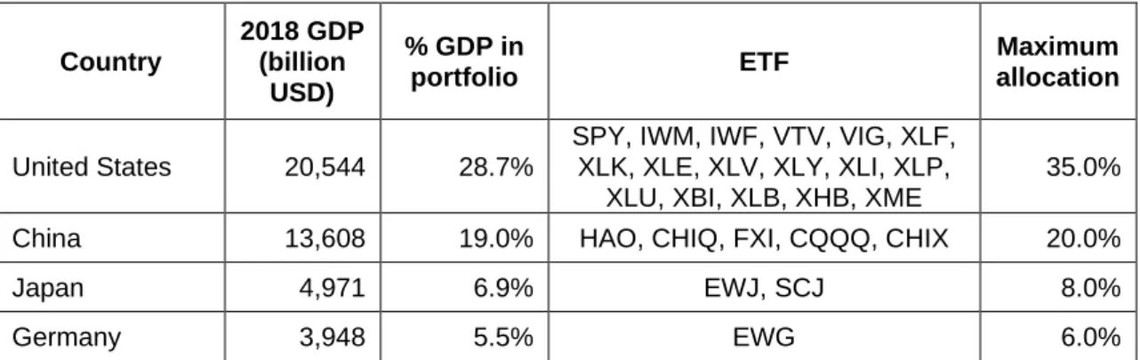
allocation to United States, which have GDP about 81 times of Vietnam or Egypt. Even though the allocation could be reasonable in term of maximizing return, it was not what we wanted for a global, diversified pension investment. Allocating a significant amount of portfolio to a single country will increase our expose to country risk. Country risk is commonly referred to the risk of foreign government declare bankruptcy, and refused to pay back its debt, but also referred to political risk, exchange-rate risk or economic un- rest. The target of a global pension portfolio is to reduce a specific risk in a country, therefore expose to country risk is not desirable. To solve this problem, we included a maximum allocation for each EF, based on the 2018 GDP of its underlying country [20].
Table 1. List of equity ETF in portfolio and their maximum allocation
Country
2018 GDP (billion
USD)
% GDP in
portfolio ETF Maximum
allocation
United States 20,544 28.7%
SPY, IWM, IWF, VTV, VIG, XLF, XLK, XLE, XLV, XLY, XLI, XLP,
XLU, XBI, XLB, XHB, XME
35.0%
China 13,608 19.0% HAO, CHIQ, FXI, CQQQ, CHIX 20.0%
Japan 4,971 6.9% EWJ, SCJ 8.0%
Germany 3,948 5.5% EWG 6.0%
United Kingdom 2,855 4.0% EWU 4.0%
France 2,778 3.9% EWQ 4.0%
India 2,719 3.8% INDY 4.0%
Italy 2,084 2.9% EWI 3.0%
Brazil 1,869 2.6% EWZ 3.0%
Canada 1,713 2.4% EWC 2.5%
Russia 1,658 2.3% RSX 2.5%
South Korea 1,619 2.3% EWY 2.5%
Australia 1,434 2.0% EWA 2.0%
Spain 1,419 2.0% EWP 2.0%
Mexico 1,221 1.7% EWW 2.0%
Netherlands 914 1.3% EWN 1.5%
Turkey 771 1.1% TUR 1.5%
Switzerland 705 1.0% EWL 1.0%
Taiwan [21] 590 0.8% EWT 1.0%
Sweden 556 0.8% EWD 1.0%
Belgium 543 0.8% EWK 1.0%
Thailand 505 0.7% THD 1.0%
Austria 455 0.6% EWO 1.0%
South Africa 368 0.5% EZA 1.0%
Hong Kong 363 0.5% EWH 1.0%
Singapore 364 0.5% EWS 1.0%
Colombia 331 0.5% GXG 1.0%
Chile 298 0.4% ECH 1.0%
Egypt 251 0.4% EGPT 1.0%
Vietnam 245 0.3% VNM 1.0%
European
market N/A N/A VGK, DFE, FDD, IEUS 4.0%
Emerging
market N/A N/A EEM 3.0%
Total 71,699 100.0% 56 ETFs 123.5%
From Table 1, we can see that the total GDP cover by countries in our portfolio is 71,699 billion USD. According to World Bank data, global GDP at 2018 is about 85,910 billion USD [20] . Our portfolio represents 83.5% of the world GDP, and exposures to the big market in North America, Europe, East Asia and emerging markets. Two countries with
significant allocation are United States and China which have a stable political and eco- nomic environment. In our current model, we use a portfolio with 60% maximum alloca- tion to equity, with the total maximum allocation of 123.5%. This allow our software to choose among 56 ETFs, with 123.5% allocation to find the optimal 60% allocation for the portfolio. The maximum allocation put a limitation on the software but leave enough room for optimization.
3.2.2 Bond and Alternative Investment Construction
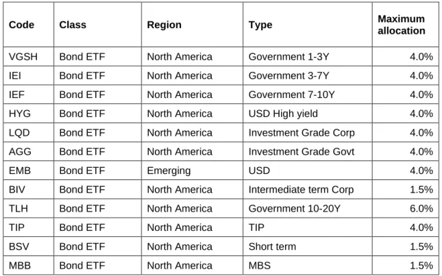
For bond ETF, we could not use the same method as equity ETF, as the number of bond ETF satisfy our condition of 10 years data is small. Also, bond ETF that cover only one country is not popular, especially in emerging countries. Bank for International Settle- ments estimated that at the end of September 2019, United States’ total debt outstanding is about 39% of the total outstanding debt [22]. And because United States debt market is dominating the world, we decided to mostly select United States bond ETF for our portfolio. Another reason is due to the low return of bond ETF, the selection of bond will not make a big different compared with equity.
Table 2. List of bond and alternatives ETF in portfolio and their maximum allocation
Code Class Region Type Maximum
allocation
VGSH Bond ETF North America Government 1-3Y 4.0%
IEI Bond ETF North America Government 3-7Y 4.0%
IEF Bond ETF North America Government 7-10Y 4.0%
HYG Bond ETF North America USD High yield 4.0%
LQD Bond ETF North America Investment Grade Corp 4.0%
AGG Bond ETF North America Investment Grade Govt 4.0%
EMB Bond ETF Emerging USD 4.0%
BIV Bond ETF North America Intermediate term Corp 1.5%
TLH Bond ETF North America Government 10-20Y 6.0%
TIP Bond ETF North America TIP 4.0%
BSV Bond ETF North America Short term 1.5%
MBB Bond ETF North America MBS 1.5%
BWX Bond ETF Non-US Government 2.5%
IEAC Bond ETF Western Europe Investment Grade Corp 1.5%
USO Alternatives Global WTI Crude Oil 3.0%
GLD Alternatives Global Gold 3.0%
SLV Alternatives Global Silver 1.0%
NIB Alternatives Global Cocoa 1.0%
VNQ Alternatives North America Real estate 1.2%
Total 55.7%
Most of bond ETF in Table 2 are investment grade and government bond, except HYG and EMB, as a result their expected return is low to trade off for their lower risk. There- fore, their allocation will not impact portfolio performance significantly. Adding alterna- tives investment such as crude oil or gold would also benefit portfolio diversification. For example, at February 2020, GLD (gold ETF) has a correlation of -0.08 with SPY (S&P 500 ETF). Negative correlation implies that adding GLD and SPY together in portfolio will lower portfolio’s variance and STDEV. At the end of 2019, there were 6 robo invest- ment accounts have miscellaneous (alternatives) investment among 64 taxable accounts reported by Backend Benchmarking [3].
3.3 Program flowchart
Bloomberg provided all historical data for our calculation. They have an API which allow us to easily extract and processing data. In our work, two most important feature of Bloomberg API is they can make price adjustment for dividend, and handle holiday dif- ferent between countries. For example, Japan have Golden Week holiday, which is na- tional holiday from 29 April to early May. Tokyo Stock Exchange will be closed during the Golden Week, therefore, any ETF listed in Tokyo Stock Exchange will not have his- torical data available during that time. The holiday problem is critical if we use daily or weekly historical data for the model but is less important if we use monthly data.
The flow of our program is illustrated by Figure 2 on page 18. Right after loading raw data from Bloomberg, our program will process them to remove any not applicable (N/A) data and convert data from string type to suitable type. There’s a function running in the background to interpret received data and converted it to reasonable value. For example,
when edit target STDEV, if user entered number 12, program will understand that user want to enter 12% or 0.12 and will store the entered value as 0.12. Data is then displayed in program’s GUI. Then at step 3, model is updated with new parameters from user input to make sure program is working with the latest information.
Figure 2. Program flowchart
After processing and editing data, user can start using program to solve for the EF (step 4: start optimization) and backtest the current portfolio (step 8 - start backtest). In each of those steps, program will perform the calculation in the background and then output the relevant chart. The chart will be the EF chart similar to Figure 1 in page 5, if user chose optimization, or the cumulative return of portfolio if user chose backtest.
Finally, program also have option to save data as csv file format. The saved data are useful in case user want to save the result of the optimization or want to share the output with clients or use it as input for other software. Save function is useful in backtest pro- cess, when users need to test their model for monthly performance from March 2015 onward. Depend on the precision setting, such backtest would take from 1 to 4 hours to complete and saving function would help users avoid running the same test repeatedly.
3.4 Program user interface
The target users of this program are investors, who familiar with economic concept but may not skilled in technology. Therefore, the program was developed with a simplified user interface. Figure 3 demonstrated the main interface when users open the program:
Figure 3. Program main interface
The main interface has three parts. The part labeled with number 1 is buttons related to step 10 (save data), step 4 (start optimization) and step 8 (start backtest) in Figure 2 page 18. The second part is where user can enter or edit their preferences. For example, user who want to take less risk can change the minimum and maximum allocation of cash in their portfolio, any change in user’s allocation will be reflected in the calculated result. The part labeled 3 is the output of the EF result. The first column represents the allocation of the highest Sharpe ratio portfolio. The remaining three columns on the right are the allocation that would result in user’s target STDEV. In this case it would be 8.5%, 9% and 9.99% from left to right.
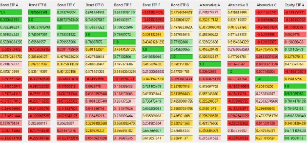
Figure 4. A screenshot of program’s correlation matrix
Program also displays correlation matrix of all portfolio’s assets (see Figure 4). To im- prove user’s ease of use, each matrix is colored based on their value. With the green color (hex color code #33cc33) for any value close to 1, the green color change to lighter green and to lighter yellow (hex color code #fff0b3) when correlation fall below 0.6. Even- tually, the cell will change to red (hex color code #ff3333) when correlation get closer to 0 or fall below 0. Program also have a horizontal scroll bar (not shown in figure) in case the correlation matrix is too long to view in one screen.
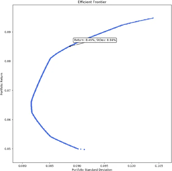
Figure 5. The Efficient Frontier result from optimization
After user click on the calculate (optimization) button, program will use available data to calculate the EF and related allocation. Aside from output the result in the main interface in Figure 3, program will also output the EF chart for user (see example in Figure 5). The chart was drew using matplotlib library, and it is an interactive chart. It keeps track of user’s mouse hover action and will display the portfolio expected return and STDEV whenever user hover the mouse over any dot in the EF. The chart help user to decide which portfolio to invest in. For example, in Figure 5, if a user prefers a higher expected return portfolio, he or she can move the mouse to the top right and select a portfolio with 9% expected return and about 10% STDEV.
Figure 6. Chart display backtest result
Another feature that would help user in his investment decision making is backtest.
Figure 6 showed an example of the result of the backtest function. From this chart, user can easily see the monthly performance of the portfolio in the past, as well as the cumu- lative result if he has invested 1 dollar at the beginning of the period. The length of the period is depending on the available data the program can get. The return from backtest is net return, which means it also includes management fees and any transaction costs.
The chart is also an interactive chart, which will display the actual return and month of any column when user hover mouse over it.
4 Improvement
The EF provides the solution for the most basic target of investment: optimized portfolio allocation to maximize return and minimize risks. Also, the Modern Portfolio Theory was
accepted as the foundation for portfolio theory since its first publication in 1952. Never- theless, the traditional Markowitz’ theory was not commonly used in practice [23]. In our model, we set the constraint of asset’s maximum allocation, partially to addressed one of the flaws of the Modern Portfolio Theory: extreme weight allocation with a small change in expected return. In this chapter, we added more improvements for our pro- gram to improve its practical use.
4.1 Semivariance
One of the main criticisms of the EF is that it uses STDEV as the measurement of risk, whereas investors in practice define risk as the probability of actual return less than the expected return. When the market is on downtrend, both STDEV and investors’ definition of risk are similar. However, when the market is on uptrend, investors will not consider the stock price moving up as risk, while STDEV will measure the upside potential as risk.
Therefore, to reflect the investors’ view better in the EF, instead of using STDEV and variance as measurement of risk, we should use semi-STDEV and semivariance to measure only downside risk. Unlike variance, semivariance only measure the variety of stock return when it is less than the expected return. Markowitz also agreed that it is more reasonable to replace variance with semivariance in his model [24, p. 476].
To implement this improvement and allow users to change between variance and semi- variance with ease, a separate function was created:
def calculateStdev(returns, rfr=0.0, isDownside=False):
"""
Determines the Stdev of the portfolio.
Parameters ---
returns: :py:class:`pandas.Series`
Daily returns of the strategy, noncumulative.
Return is in form of r% (not 1 + r%) rfr: :class:`float`, optional
minimum acceptable return, expected return isDownside: :class:`bool`, optional
If True, will calculate downside risk instead of STDEV Returns
---
:py:class:`pandas.Series`
Stdev of the portfolio """
if (isDownside):
print('Calculating semivariance instead of variance') downsideReturn = (returns - rfr)
mask = downsideReturn >= 0 downsideReturn[mask] = 0 return downsideReturn.std()
return returns.std()
Listing 2. Python function to calculate STDEV or semi-STDEV (downside risk) depend on user’s input
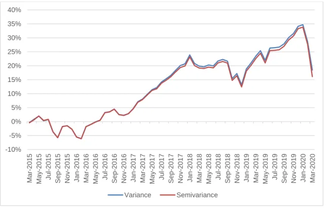
For our case, risk free rate was chosen as expected return. If user selects semivariance in setting, semi-STDEV will be calculated instead, and any return higher than expected return will be ignored in the STDEV calculation. Then program will use the result of semi- STDEV to calculate portfolio semivariance in next step. We backtested the semivariance model from March 2015 to March 2020, using 5 years historical data from February 2010 and obtained the result in Figure 7:
Figure 7. Cumulative gross return of Sharpe portfolios using variance and semivariance -10%
-5%
0%
5%
10%
15%
20%
25%
30%
35%
40%
Mar-2015 May-2015 Jul-2015 Sep-2015 Nov-2015 Jan-2016 Mar-2016 May-2016 Jul-2016 Sep-2016 Nov-2016 Jan-2017 Mar-2017 May-2017 Jul-2017 Sep-2017 Nov-2017 Jan-2018 Mar-2018 May-2018 Jul-2018 Sep-2018 Nov-2018 Jan-2019 Mar-2019 May-2019 Jul-2019 Sep-2019 Nov-2019 Jan-2020 Mar-2020
Variance Semivariance
From the backtest result above, we can see that variance and semivariance portfolio have similar performance. And variance portfolio in fact has higher return than semivar- iance portfolio. Even when excluding the February 2020 and March 2020, two outlier months when the global coronavirus pandemic happen, variance portfolio has 34.697%
return, which is 0.86% higher than semivariance portfolio. There were a few months that semivariance portfolio performed slightly better than its counterpart, and there were months, especially during 2018 and 2019, that we can clearly see variance portfolio was better. Two portfolios have performed nearly identical to each other during the tested period, with monthly correlation was 0.99816. Variance portfolio, in this case, is as prac- tical as semivariance. Refer to Markowitz’s article about semivariance, he also men- tioned that he found mean-variance model can provide an sufficient estimate for ex- pected return as mean-semivariance [24].
Another study of semivariance were published by Aleksei Tcysin and Pivovarov Dmitrii from Lapland University of Applied Sciences [25]. Their work was studied to has better understanding of the benefit of semivariance in Modern Portfolio Theory. In their thesis, author studied the performance of semivariance model and compared it with variance model and SPY ETF (tracking the S&P 500 Index). They tested the model with three different environments: bull market (2014), bear market (2008) and sideway market (2015) and the results show that while semivariance portfolio outperform variance and SPY in 2014 and 2015, but it underperformed in 2008. The authors concluded that while the combination of semivariance and Bayes-Stein estimators generally produce superior results, they cannot identify the source of the exceed return is semivariance or Bayes- Stein estimator framework. They also noted that the model needs further testing and research before putting in practice.
There were several differences in Tcysin and Dmitrii model when compared with the model used in this thesis, which could explain the difference. First, the authors used Bayes-Stein estimators, while we did not. Second, they used 30 stocks representing Dow Jones Industrial Average for testing, which is a 100% equity portfolio, while our portfolio has a maximum allocation of equity of 60%. Lower allocation to equity would result is lower volatility and as the result the different between variance and semivariance portfo- lio would be smaller. Our portfolio also has maximum allocation for each ETF, which increases the diversification in portfolios and lowers their volatility. Another point is that
Tcysin and Dmitrii tested their model with different level of risk tolerance, and the higher the risk tolerance, the larger the difference. With risk tolerance of 0, the difference in return between variance and semivariance was lowered to 2.1% in bullish market. And finally, instead of testing only for one market condition, we test 5 years performance from March 2015 to March 2020, during that period two portfolios experienced bull market, bear market and sideway market. The difference in performance in bull market condition could be offset by bear market followed it.
Nevertheless, semivariance improvement added to the program could help users im- prove their portfolio performance. Users, however, need to understand that semivariance portfolio does not always outperform variance portfolio. Also, they need to perform their own backtest research, which is also available as a function in the program, thoroughly with their target return and risk to see which model performed better.
4.2 Black-Litterman model
In our model, equity portfolio is defined as all ETFs listed in Table 1, bond portfolio and alternatives investments are listed in Table 2. The BL’s market portfolio is the portfolio formed by combine 60% equity portfolio and 40% bond and alternatives portfolio. The ratio 60%/40% is the constraint in our pension investment strategy during the backtest process. The market portfolio, regardless of its allocation, also follow the same con- straint. While the market capitalization data of each ETF is available in Bloomberg, their historical data is not. For this reason, we used the fund total assets data instead. Be- cause ETFs are designed to track their underlying assets, the different between ETFs’
market capitalization and their total assets is negligible. We can calculate matrix multi- plication using NumPy’s matmul function. Listing 2 show a simplified version, without debug code and error handling, of the program’s Black-Litterman model.
import numpy as np import pandas as pd
def blackLitterman(cagr, stdev, correlation, rfr):
"""
Calculate Black-Litterman model’s implied equilibrium return Parameters
---
cagr: :class:`pandas.Series`
Expected return of all assets in portfolio
stdev: :class:`pandas.Series`
Stdev of all assets in portfolio correlation: :class:`pandas.DataFrame`
Correlation matrix of all assets on portfolio rfr: :class:`float`
risk free rate Returns
---
:py:class:`pandas.Series`
Implied equilibrium returns matrix from Black-Litterman model """
# Calculate market weight matrix using a helper function portWeight = calculateMarketCapWeight()
# This code helps match each asset with its return, stdev and weight dataBL = pd.DataFrame({'Return':cagr, 'Stdev':stdev,
'Weight':portWeight.iloc[:,0]}, index = cagr.index)
# Calculate portfolio return
portReturn = sum(dataBL.Return*dataBL.Weight)
# Calculate portfolio covariance matrix using a helper function portCov = calculateCov(correlation.values, stdev)
# Calculate portfolio risk using weight matrix and covariance matrix portRisk = np.matmul(dataBL.Weight.transpose(), portCov)
portRisk = np.matmul(portRisk, dataBL.Weight)
# Calculate risk aversion coefficient riskAversion = (portReturn - rfr)/portRisk
# Calculate implied equilibrium return
equiReturn = riskAversion*np.matmul(portCov, dataBL.Weight)
# Convert result to pandas.Series format
equiReturn = pd.Series(equiReturn[:,], index = cagr.index)
return equiReturn
Listing 3. Simplified version of Black-Litterman model in the program.
The helper function calculateMarketCapWeight will need fund total assets data from Bloomberg when it calculates weight matrix. We use helper function calculateCov in- stead of NumPy’s cov function to calculate covariance matrix, as it allows user to choose semivariance option for the model. Whenever user start the optimization process, pro- gram will check if Black-Litterman model is selected. If it was, then the program will first run the blackLitterman function to calculate equilibrium return and use that in the optimi- zation model. Otherwise, the program will use historical 5-year CAGR as expected return instead.
Figure 8. Cumulative gross return of Sharpe portfolios using variance and Black-Litterman The performance of two Sharpe portfolios, one calculated using traditional return-vari- ance method, and other using equilibrium return from BL model can be seen in Figure 8.
Semivariance method was not included in the figure because its performance is closely represented by variance portfolio. Although BL portfolio failed to compete in the end of 2015 and first quarter of 2016, it recovered quickly and outperformed the variance port- folio during the bull market period after that. And it yielded higher return for the entire year of 2019. Another important period is the 1st quarter of 2020, when the coronavirus pandemic reached outside China. At January and February 2020, BL performance was higher than variance portfolio, however, during March 2020 when the number of daily cases in United State and European countries increased significantly [26], BL portfolio actual return was -11.222% (while variance portfolio has return of -7.842%). Looking at the allocation in appendix 1, we found the reason is due to BL model allocation more equity United States and European countries. The economic downturn due to corona- virus was an outlier event that rarely happen, with the closest event can related to it is the Great Depression in 1930s [27]. If we remove the 2020 performance for this reason, we can say that during the period from March 2015 to December 2019, Black-Litterman portfolio has outperformed traditional variance portfolio.
-20%
-10%
0%
10%
20%
30%
40%
Mar-2015 May-2015 Jul-2015 Sep-2015 Nov-2015 Jan-2016 Mar-2016 May-2016 Jul-2016 Sep-2016 Nov-2016 Jan-2017 Mar-2017 May-2017 Jul-2017 Sep-2017 Nov-2017 Jan-2018 Mar-2018 May-2018 Jul-2018 Sep-2018 Nov-2018 Jan-2019 Mar-2019 May-2019 Jul-2019 Sep-2019 Nov-2019 Jan-2020 Mar-2020
Variance Black-Litterman
As mentioned in chapter 2.4, during the backtest process, we cannot use investor’s view as an input. The result we obtained is the BL model without investor’s view. In practice use, however, program allow investors to input their view of future performance, and their confident level of the views in the model. Users need to perform their own backtest to see the impact of their views to the portfolio performance, as their forecasts may not correctly reflect the actual result of the market.
4.3 Portfolio Simplification
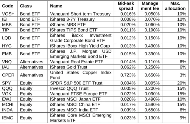
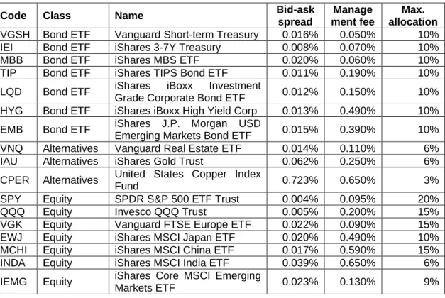
Up until this section, portfolio return was calculated without including any fees, i.e. gross return. In practice, when invested in ETFs, investors must pay at least 3 types of fee:
commission fee, management fee and bid-ask spread. Commission fee is the fee inves- tors must pay to their stockbrokers for processing their purchase or sales of ETFs. This fee varies depend on the stockbrokers and is often based on the total value of the trade.
Management fee is fee collected by the ETFs management company to cover for admin- istration cost. Generally, for tracking ETFs, the bigger the fund assets value, the smaller the percentage of the fee. Bid-ask spread is the different in the price the buyer willing to pay (bid) and the price the seller want to accept (ask). High bid-ask spread will cost investors when they want to trade their ETFs. For example, ETF with bid-ask spread of 1% mean that investor purchase the ETF with $100, when immediately sell them back can only get $99. ETFs with high trading volume will have lower bid-ask spread, while illiquid ETFs will have higher spread.
Our portfolio has 75 ETFs, among those ETFs, there are ETFs have higher fee than other. For bid-ask spread, we have EGPT (5.677%) and GXG (3.997%). IWM have 1.19% management fees, while SPY has only 0.095% and United States Select Sectors ETF (XLF, XLK, XLE …) have 0.03% to 0.035% annual fee. When including fee in return calculation, i.e. net return, we found a significant amount of portfolio return was offset by fees. While the portfolio is suitable for studying the effect of different market condition and model, it is not applicable in real investment world. Instead, we composed a simpli- fied version of portfolio, with target to replicate the global portfolio, while focus on ETFs with lower fees. Details of portfolio is listed in Table 3 below: