The first describes the properties of the ISC analysis and ISCtoolbox for Matlab implementation. The spatial smoothing turned out to be a mandatory preprocessing step for the ISC analysis.
Basics of Functional Magnetic Resonance Imaging
The correlation between the increased oxygen consumption and firing of neurons was proven in the studies of Mukamel et al. Due to the indirect nature of the BOLD measurement, there is a 2-6 second delay between the BOLD response compared to the actual neuronal activity.
Functional Magnetic Resonance Imaging Data Analysis
In model-based analyses, it is crucial to consider this delay in addition to other physiological properties of the BOLD signal (Logothetis, 2003; Poldrack et al., 2011).
Objectives
Motivation
Structure of The Thesis
GLM and ISC analyzes are described in detail in Chapters 3 and 4. The details of the data processing pipeline here follow the description of Poldrack et al. 2011) and the typical pipeline used by the FMRIB Software Library (FSL) package (Jenkinson et al., 2012). Smith et al., 2004) and SPM software (Friston, 2008) have different nomenclature and a different order for normalization, smoothing, and statistical analysis.
Common Processing Steps
The normalization also typically requires less computing resources with a single statistical three-dimensional (3D) volume compared to the multiple volumes of the fMRI data (Poldrack et al., 2011; Smith et al., 2004). In this thesis, the selected software was FEAT GLM analysis software (Beckmann et al., 2003; . Woolrich et al., 2004) from FSL software package and ISCtoolbox for Matlab (Kauppi et al., 2014).
Analysis Dependent Processing Steps
As a term, the spatial normalization refers to the procedure of recording the data from the original spatial space to a common template and thus to a common space of the template. Then the affine transformation received from the registration of the MRI image to the common template is applied to the fMRI data that was registered to the MRI image.
Data Analysis and Post-processing
In ISC analysis, the measurement of brain activity is based on the similarity of the corresponding time courses within a group of subjects. Panel (d) presents the 37 STRONG time courses obtained by peaking the ISC analysis of the VG task in Pajula et al.

General Linear Model Analysis
The group-level GLM analysis is applied with the same principle as the first-level analysis, but the input to the model fitting is now the estimates of the fitted first-level models for each subject included in the study. In general, two methods are common when modeling the base model interfaces at the group level.
Multiple Comparisons Correction
For this reason, Bonferroni-corrected thresholds are typically overly conservative with fMRI data (Poldrack et al., 2011). It has been argued that studies with naturalistic stimuli can reveal the brain functions involved in everyday encounters (Hasson et al. Jääskeläinen et al., 2008).
Inter-subject Correlation Analysis
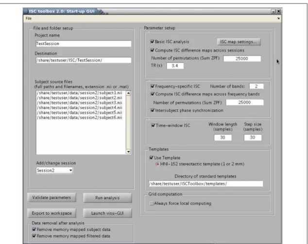
Unlike ICA, the ISC analysis looks for the similarity of the corresponding time series within the group of subjects. ISCtoolbox for Matlab1 (Kauppi et al., 2014) is an open source software implementation of the ISC analysis.

Computational Considerations
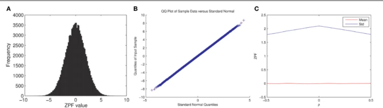
First, a Z-transform is applied to the correlations and then paired Fisher's Z-transform (ZPF) (Raghunathan et al., 1996) statistics are calculated from them. At the end, the paired ZPF statistics are combined into a sum ZPF statistic (see details from Kauppi et al.
Parallel Implementation of ISCtoolbox
The second part of the parallelization system is the waiting mechanism for the triggered processes. When all processes of the current step have been submitted, the master process passes the collected process IDs to the waitGrid function.

Materials
Properties and validation of inter-subject correlation analysis The detailed descriptions of the stimulus and the data used in this thesis can be found in Pajula et al. The main reason subjects had to just think about the response on the tasks where a response was required was that speech could cause challenging motion artifacts to the data. According to Rosen et al. 2000) thinking causes more or less the same activation in the brain than speaking the same output aloud.
The described stimulus design allows for easy analysis with a boxcar model to find brain areas involved in the described activity. The main limitations of FRB and similar models are that in everyday life the brain does not have this simple limited type of stimulus, but an extremely complex combination of stimuli of all kinds. For this reason, these types of studies cannot show exactly how the individual brain works in everyday life situations, and more complex stimulations such as naturalistic stimulation are needed.
Tests with Simulated Data
Comparison Studies
Properties and validation of inter-subject correlation analysis this issue should be carefully considered when designing the pretreatment. The smoothing kernel should be chosen large enough that the required SNR is archived, but small enough to minimize the number of possible false positives.
The Effects of Sample Size
ISC Toolbox version 2.0 was published with the publication and the ISC Toolbox 2.1 was published shortly after. The version 2.1 was published due to usability problems with parallel environments as discussed in Section 5.3.
Publication 2
Publication 3
The results also showed that the 2.5 voxel width of the Gaussian smoothing kernel can produce suitable results with the ISC analysis.
Publication 4
Author’s Contribution to the Publications
Within this thesis, the accuracy of the ISC analysis and the properties of ISCtoolbox have been investigated from several aspects. The validation of the ISC analysis was performed by comparing the accuracy of the ISC analysis with a typical group GLM analysis. The studies in this thesis focus on the critical questions about the accuracy and properties of the ISC analysis and the implementation of ISCtoolbox.
In practice, the ISC analysis detects the similarities in the BOLD response across a group of subjects, but cannot separate the influence of specific aspects of the stimuli. It was speculated that these areas were a result of inter-subject time course synchronization, which did not follow the structure of the stimulus model used in the GLM analysis. When considering the properties of the BOLD signal, the Gaussian spatial smoothing can be envisioned as a natural choice for a denoising method for ISC analysis.
In ISC analysis, the amount of smoothing required depends on the accuracy of subject registration and the SNR of the data. If the co-registration of the subjects is good, less spatial smoothing is required to ensure the spatial overlap of the subject data, and the size of the smoothing kernel can be largely chosen to ensure sufficient SNR. This is natural since for a successful ISC analysis it is essential to have common stimuli for the entire subject group, high-quality alignment with the common spatial domain, and sufficient SNR of the data.
ISCtoolbox Implementation
Even a moderately parallel environment can significantly speed up the overall computation, which is represented in the Figure 8.2 (Kauppi et al., 2014). As shown in Figure 8.2, the parallel cluster environments can significantly speed up the ISC analysis and in the future the parallel support will become even more important when the size and length of the data increases. It is reasonable to assume that the grid engine support of ISCtoolbox will become even more attractive to the researchers in the future.
Although parallel patches are typically used in a cluster environment, they also allow somewhat large computations to be performed locally on modern high-end desktop computers. With a cluster, individual resampling corrections are applied in parallel processes, but in a local environment they are calculated sequentially. In ISC analysis, each subject acts as a model for each other, which prevents all data from being stored simultaneously in the GPU memory.
As memory increases and a larger instruction set becomes available in GPE hardware, it may be possible to leverage the power of GPGPU hardware in ISC analysis. ISC analysis could be used with GPU or Phi hardware in the future, but in practice would require a lot of optimization for toolbox memory usage. These systems should be considered in future development of the ISCtoolbox and possible support for pipeline software should be considered.

Open Data and Data Sharing
K., “Fundamentals of a robust functional magnetic resonance signal,” The Journal of Neuroscience, vol. ISC tools allow analysis of time-course similarities across multiple subjects. The GUI enables fast and comprehensive visualization of ISC analysis results in an exploratory way.
GLM and ISC analysis results for the AN task. Distribution (a) shows voxel-wise statistical values of GLM (horizontal axis) and ISC (vertical axis). Most of the values are concentrated near the origin, which is not visible in the scatterplot. Thus, the ISC analysis was more conservative of the two methods especially with the lower q value.
The color coding in the images is the same as in Figure 3 of the article. Thus, the ISC analysis was the more conservative of the two methods, especially with the lowest q value. In [5], a Gaussian filter with 5 mm full width at half maximum (FWHM) was used for spatial smoothing according to the requirements of the GLM analysis.
The top half of the matrix represents ISC (blue triangle) and the bottom half represents GLM (red triangle). We compared the split-half analysis ISC statistical maps against the following criteria. The temporal location of the decline was in the middle of the time series (𝑡 = 172s, excluding stabilization volumes).
Bowley, “Standard deviation of the correlation coefficient,” Journal of the American Statistical Association, vol.