[PENDING] Application of Global Sensitivity Analysis of Model Output to Building Thermal Simulations

(1)

Application of Global Sensitivity Analysis of Model Output to Building Thermal Simulations

Thierry Alex MARA ⁽¹⁾ , Stefano TARANTOLA⁽²⁾

(1) University of Reunion Island, L.P.B.S. (EA 4076), Faculty of Human and Environmental Sciences, 117 Rue General Ailleret, 97430 Tampon, La Réunion – France.

Tel : +262 262 93 82 12 Fax : +262 262 93 86 65

corresponding author, email : mara@univ-reunion.fr

(2) Institute for the Protection and Security of the Citizen, Joint Research Centre, European Commission, TP361, IPSC, Via E. Fermi 2749, 21027 Ispra (VA), Italy.

email stefano.tarantola@jrc.it

(2)

ABSTRACT

In this paper is exposed a set of applications of global sensitivity analysis to building thermal modelling. The aim is to demonstrate the interest of such tools for model analysis and to encourage their use. Indeed, since the last ten years important improvements have been made in the field of sensitivity analysis and especially in ANOVA-based computational methods. Yet, their use in the field of building performance modelling is uncommon. After recalling the concept of ANOVA- based sensitivity analysis and the associated sensitivity indices, we describe some computational methods to compute the global sensitivity indices of model input factors. The emphasis is put on the methodology that is computationally cheapest but provides the more information. For illustration, they are applied to an actual test-cell thermal model.

Keywords: global sensitivity analysis, analyse of variance, design of experiments, generalized additive model, model calibration, building thermal model

(3)

With the increasing power of computers and their low cost, the 90's have favoured the development of computer models. In building physics, numerous computer-aided programs have been proposed to professional and engineers for improving building energy efficiency. Indeed, computer models can help the designer in the choice of the optimal designs and appropriate materials as well as sizing devices in order to improve the occupants comfort or minimize the electrical consumption. Their intensive use has encouraged the community of building physics to derive standard procedures to increase confidence in the softwares results.

The aim of this paper is to demonstrate that global sensitivity analysis (GSA) of model output can help both the users and modellers. GSA aims at establishing how the variation in the model output can be apportioned to different sources of variation. Although great improvements have been brought to the computational methods for GSA since the last decade, their use remains rare in the field of building energy simulation [1,2,3,4]. Conversely, local sensitivity analysis and the one-at-a- time approach are mostly employed even though, to our point of view, such analyses are less reliable [5,6,7].

After recalling some general concepts of GSA and the basis of ANOVA-based sensitivity analysis, we describe some computational methods to estimate the sensitivity indices. Then, we apply them to the building thermal model of an existing test cell by investigating the test cell components that are responsible of the variation of the indoor air temperature. On a second phase, we show that GSA is very useful for diagnosis of modelling errors when an empirical validation work is undertaken.

2 Generality about sensitivity analysis

Computer models are generally employed for decision-making purposes or to have a deeper insight of the process of interest. They may be used to predict future outcomes under different assumptions or to characterize a process once measurements are available. So without loss of generality, we can

(5)

state that a model is composed of a set of inputs that govern the model responses and relies on a set of equations and assumptions. Whatever the objective, it is crucial to account for uncertainties in the model inputs (including alternative assumptions and different ways to model the underlying system) and assessing their impact on the output of interest. This is the role of uncertainty and sensitivity analysis of model output. It is important to note that the latter should not be necessarily the model response per se but the question that the model has been employed to answer [8].

Let us denote by F(X) the response of a computational model and X = {X1, X2…, Xk} the set of uncertain model inputs, i.e. all the uncertain quantities in the system under analysis that can have an influence on the model response. This may include model parameters (scalar or functions of time and space), sub-models (when alternative modelling structures or equations are plausible), alternative assumptions or forcing functions, and so on. Consequently, each uncertain model input can have continuous or discrete values, and can be a scalar or a function of time and/or space.

Given the uncertainty of the inputs, one can be interested in assessing the uncertainty in the model response (uncertainty analysis) and eventually identify the inputs that contribute the most to that uncertainty (sensitivity analysis). Uncertainty analysis is useful to investigate the reliability of the model. Indeed, the model is useful (i.e. reliable) only if the uncertainty interval of the response is narrow enough. On the other hand, sensitivity analysis allows to point out the inputs that contribute the most to the model response variation. Priority should then be given to the reduction of the uncertainty of those inputs for which uncertainty can be reduced (epistemic uncertainty) by gathering more data for that input, if possible, or through estimation via indirect measurements.

This will finally improve the accuracy of the predictions. Such analysis is known as model input prioritization [9,10], as it establishes priorities for future research.

Sensitivity analysis can also be used for model simplification, to identify the inputs to which the model response is insensitive. The identified inputs can then be fixed at any value over their uncertainty range without any effect on the model response. One can also be interested in

(6)

specified range (see [10] for a review of settings that can be addressed with SA).

3 Global sensitivity analysis

3.1 ANOVA-based sensitivity analysis

Local sensitivity analysis evaluates the influence of uncertain inputs around a point in the input space and generally relies on the estimation, at this point, of the partial derivatives of the output with respect to the inputs. This is known as a one-at-a-time measure of sensitivity because it measures the effect on the response of varying one input alone by a fixed fraction of its value (assumed known). As a consequence, if the model is non-linear, the relative importance of the model inputs depends on the chosen point. Several investigators tried to get around this limitation by evaluating averages of the partial derivatives at different points in the input space (see for example the screening method proposed by [11], and later optimized by [12]).

Conversely, global sensitivity analysis of model output evaluates the relative importance of inputs when they are varied generously, i.e. when their uncertainty is acknowledged over a wide range.

One approach to GSA is the ANalysis Of VAriance of the model response [13]. In the ANOVA- based sensitivity analysis non-linearity in the model is not an issue, the approach can capture the fraction of the model response variance explained by a model input on its own or by a group of model inputs. In addition, it can also provide the total contribution to the output variance of a given input, that is its marginal contribution and its cooperative contribution.

Using ANOVA for sensitivity analysis may fail if the density distribution of the output is far from normality. In such case, indeed, the second-order moment alone is not able to describe the model output uncertainty. Sensitivity analysis methods based on the whole distribution of the model output have also been proposed [14] and are object of ongoing research [15], but they are computationally expensive. So in the following, we will exclusively discuss the ANOVA-based methods for models with independent inputs, assuming that the uncertainty of a model response is fully described by its variance. There are different computational techniques to perform sensitivity analysis using

(7)

ANOVA: we will focus on those based on the work of Sobol’ later extended by Saltelli [13,16]. The reader interested in the other approaches is invited to read Saltelli et al. 1999, Rabitz et al. 1999, Morris 2006, Oakley 2004, Sudret 2008 and Tarantola et al. 2007 ([17,18,19,20,21,22] resp.).

GSA treats the model under consideration as a black-box. The investigation is performed by the following steps:

1) Select the model and the question of interest ,

2) Select the uncertain model inputs (k) and set their probability density functions, 3) Generate a sample of the model input space of size N (i.e. an Nxk matrix), 4) Run the model for each sample point and save the responses,

5) Perform UA/SA on the response of interest and interpret the results.

In step one, the selection of the question of interest should allow the analyst to answer the problem at hand properly. In step two, all inputs that are subject to uncertainty are selected. Assigning a density distribution to unknown inputs is not an easy task and may require expert involvement. Yet, the wider the uncertainty associated to a model input, the more likely its influence on the model output. Generally, when no a-priori information is available, the uncertainty range is selected large enough so as to be plausible and a uniform density distribution is assumed. In step three, the different combinations of input values are generated accordingly with their density distribution and the sample matrix is stored in a file. This task can be more challenging when model input are correlated. In step four, the different trials are then employed to run the model. This step may require large computational time, depending on the complexity of the model under analysis. So, in general the affordable number N of model simulations is derived from the total computational budget available. The computer code has to be designed so that the model is executed N times in a loop where, each time, a new point of the input space is fed into the model. Developers of end-users programs in building energy simulation are encouraged to include a sensitivity analysis module in their codes (Fürbringer et al. [23]). Finally, UA and SA are performed in the fifth step (see next

(8)

necessarily the model output per-se, but a function of it. For instance, the program may predict the indoor air humidity, temperature and air velocity. These predictions may allow the evaluation of the thermal comfort of occupants, which can be the response of interest.

A variety of software packages exist for the generation of input samples as well as to perform both UA and SA. While in this paper we employ SimLab (see [24]), a comprehensive list of such tools is available in [25]. For UA, the density distribution or the cumulative distribution can be plotted as well as the estimated confidence bounds. As far as SA is concerned, quantitative sensitivity indices of the inputs are estimated as we see in the next section.

3.2 ANOVA-based sensitivity indices

Sobol' [13] proves that any square integrable mathematical function can be decomposed as follows:

FX=f₀

∑

i=1 k

f_iX_i

∑

ji k

f_ijX_i, X _j...f_12...kX_1,X_2,..., X_k (1)

with, E[f_i₁_..._i_sX_i₁,..., X_i_s]=0 ∀ {i1...i_s}⊆{1,2,..., k} , where E[.] is the expectation operator.

This decomposition is unique only if the functions are pairwise orthogonal, that is, E[f_i

q...i_tX_i

q,..., X_i

tf_i

r...i_sX_i

r,..., X_i

s]=0 ∀i_r...i_s≠i_q...i_t

which is ensured by the assumption of independence among the inputs . As a consequence, E[FX]=f₀ ,

E[FX∣X_i]=f₀f_iX_i ,

and E[FX∣X_i, X _j]=f₀f_iX_if _jX _jf_ijX_i, X _j , ...

E[.|.] is the conditional expectation.

It comes that the variance of F can be decomposed in a sum of fractional variances:

D=

∑

i=1 k

D_i

∑

ji k

D_ij...D_12...k

where D = V[F(X)] is the total variance of F, Di = V[fi(Xi)] is the marginal variance of Xi and

(9)

D_i

1...i_s=V[f_i

1...i_sX_i

1,..., X_i

s] is the cooperative fractional variance of {X_i

1,..., X_i

s} and is induced by interactions between the inputs {X_i

1,..., X_i

s} . For convenience, the previous equivalence is rewritten as follows:

1 =

∑

i=1 k

S_i

∑

ji k

S_ij...S_12...k (2)

where ^Si₁...i_s=D_i₁_...i_s/D is the so-called global sensitivity index (also called main effect) . S_i=V[E[FX∣X_i]]

V[FX] =D_i

D is the first-order sensitivity index that measures the amount of the response variance explained by Xi alone,

S_ij=D_ij

D is the second-order sensitivity index that measures the amount of the response variance explained by the interaction between Xi and Xj and so on. It is sometimes convenient to introduce the closed-sensitivity index defined by:

S_ij^c=V[E[FX∣X_i, X_j]]

V[FX] =D_iD_jD_ij

D =S_iS_jSij that measures the main effect of the group of factors {Xi, Xj}.

A sensitivity index that has an important role in factor fixing setting (see [10]) is the total sensitivity index defined by:

ST_i=E[V[FX∣X_−i]]

V[FX] =

D_i₁

∑

i2i1

k

D_i₁_i₂

∑

i3i2i1

k

D_i₁_i₂_i₃...D_12...k D

where X-i = {X₁, X₂, ..., X_i-1, X_i+1, ..., X_k}.

This index accounts for all contributions of Xi to the variance of F(X) so that if STi is close to zero, Xi can be deemed as non significant. Consequently, the input can be fixed at any value in its uncertainty range without changing the response (model reduction).

The computational cost of evaluating all the sensitivity indices (i.e. 2^k-1) is prohibitive. In practice, only S and ST are estimated because they summarize the essential information. Eq. (2) yields the

(10)

following classification of input/output relationships in a model: if

∑

i=1

k S_i=1 , then S_i = ST_i for all i in [1,k] and the model is said additive (linear models are special cases of additive models);

otherwise, the model is said non-additive and STi ≥ Si.

3.3 Design of experiments and ANOVA

The methodology of the designs of experiments (DOE) is probably at the origin of sensitivity analysis of computer models. Even though it was originally introduced for laboratory experiments [26], it has been extended to the analysis of computers [27-28] and was widely used for this purpose [29,30,1,3,19]. Different designs of experiments are proposed in the literature, like the full factorial designs, fractional factorial designs, supersaturated designs and so on ...

For example, the two-levels full factorial design relies on the approximation of the model by a polynomial expansion of the form:

FX=0

∑

i=1 k

ix_i

∑

ji k

ijx_ix_j...12...kx₁x₂...x_k (3)

where the xi's are the standardized inputs and the 2^k coefficients bi's are unknown. To determine the bi's, the input factors are assigned two discrete values (levels), usually -1 and +1. Then, the model response is evaluated for all the 2^k possible combinations of the input levels and the polynomial coefficients are estimated straightforwardly by solving the system of 2^k equations. The two-level full factorial design assumes that the density distribution of the xi's is :

px_i=1

2 x_i−11

2 x_i1 (4)

where, d(x) is the Dirac distribution and x_i=X_i– E[X_i]



^^V^[^Xⁱ^] is the standardized variable.

Eq.(3) is an ANOVA-decomposition because, E[x_i₁...x_i

s]=0 ∀ {i₁...i_s}⊆{1,2,..., k} , E[FX]=0

(11)

and E[x_i

q...x_i

tx_i

r...x_i

s]=

{

^{0 if,}^{1 if,}ⁱⁱ^r^r^...i^...i^s^s⁼^≠ⁱⁱ^q^q^...i^...i^t^t ^.

Then, it is straightforward to prove that D_i₁_...i_s=_i²₁_...i_s from which can deduce the link between the bi's and the ANOVA-based sensitivity indices. Because of the assumed density distribution of the inputs, DOE is generally employed for screening purposes, thanks to their low computational cost and capability to estimate qualitative measures of importance. For this exercise, the iterated fractional factorial design, introduced by Andres, is particularly efficient [29].

4 Numerical methods for UASA

4.1 Latin hypercube sampling for uncertainty analysis

UA of model output is achieved with Monte Carlo analysis, which is based on multiple evaluations of the model for random sets of inputs. This requires that the input values be randomly sampled accordingly with their respective probability density function. The accuracy of the analysis strongly depends on the sampling technique that must ensure a good coverage of the input space. The latin hypercube sampling technique (LHS) covers better the input space than random sampling [31].

LHS is based on the following steps, for each input (see Fig. 1):

– compute their cumulative distribution,

– divide their uncertainty ranges into r contiguous intervals of equal probability,

– for each input, randomly select a value in each interval (r values per input),

– randomly create r combinations with the selected factors values,

– restart the procedure until N trials are obtained.

Such a procedure guarantees independence between the inputs as well as the respect of the marginal probability distribution and the good coverage of the input space. Besides, the procedure of Iman &

Conover coupled with LHS allows to generate correlated samples (see [32,33]).

The uncertainty analysis of the response of interest is achieved by plotting either its density

(12)

distribution or its cumulative distribution. The former provides, for instance, the most probable response whereas with the latter makes easy to estimate confidence intervals (see Fig. 2).

[Insert Fig. 1 about here]

4.2 Computing the first-order sensitivity indices

A variety of techniques is available to evaluate the first-order sensitivity measures, among which we find one derived from the generalized additive model (Hastie and Tibshirani [34]). This technique provides estimates of first-order sensitivity indices using a single sample of inputs (see Mara et al.

[4]), and consists in approximating f_i(X_i) in the ANOVA-decomposition by a polynomial or some other function. For each input, the approximation is achieved by fitting the model response Y on a polynomial of the form:

P_iX_i=a_i,0a_i,1X_ia_i_,2X_i²⋯a_{i , M} X_i^M , ∀i=1,2,..., k where M is the polynomial order (usually less than 5) and the ai,j's are estimated by least squares. Then, the first-order sensitivity indices are computed as follows:

S_i=V P_iX_i

V FX (4)

where V. is the variance best unbiased estimate.

The sensitivity indices for the other inputs are estimated independently using the same sample. Note that, if a first-order polynomial is chosen (M = 1), then S_i would represent the fractional variance of the model response explained by its linear relationship with X_i, i.e. it would equal the square of the correlation coefficient between X_i and F(X), which is the same as the square of the standardized regression coefficient (SRC). This result explains why the SRC is so popular for SA. However, SRCs are not reliable when the model is non monotonic.

(13)

4.3 Computing higher-order sensitivity indices

To compute ANOVA-based sensitivity indices, Sobol’ [13] proposed a general sampling strategy that later, was improved, in terms of computational cost, by Saltelli [16] and, in terms of accuracy, by Sobol’ et al. [35]. The procedure of Sobol’ relies on the generation of two samples of size N. The first one X⁽¹⁾ is the reference matrix , the second one X⁽²⁾ is generated from the reference and depends on the sensitivity index to be estimated. Fig. 3 sums up the different possibilities. Note the specificity of the Sobol' strategy, which enables groups of inputs to be treated as individual inputs.

The two sample matrices produce two vectors of model responses, respectively noted as F(X⁽¹⁾) and F(X⁽²⁾), from which one of the following sensitivity indices can be estimated as:

S_i= FX^2, FX^1 ,

ST _i=1 − FX^2, FX^^1 , (5) S_ij^c= FX^2, FX^1 , ... (6) where .,. is the estimated correlation coefficient (or standardized regression coefficient). The original numerical computation of the sensitivity indices differs from the one proposed here. But, it has been tested (not shown) that, for the estimate of STi, the proposed numerical calculation is particularly accurate and has the advantage to only requires one sample set per index (given the reference set).

5 Applications to a test-cell thermal model 5.1 The test-cell and its thermal model

In this section, ANOVA-based GSA is employed for a better characterization and understanding of the thermal behaviour of an actual test cell. The latter is set on an experimental platform at the

(14)

University of Reunion Island. It was built for model validation and device testing purposes.

Experiments have been performed in the past to calibrate the thermal model and to validate a model of HVAC system (see [36,37]). Here, the model calibration is revisited by applying GSA and the building components that are mainly responsible of the variation of indoor air temperature are identified.

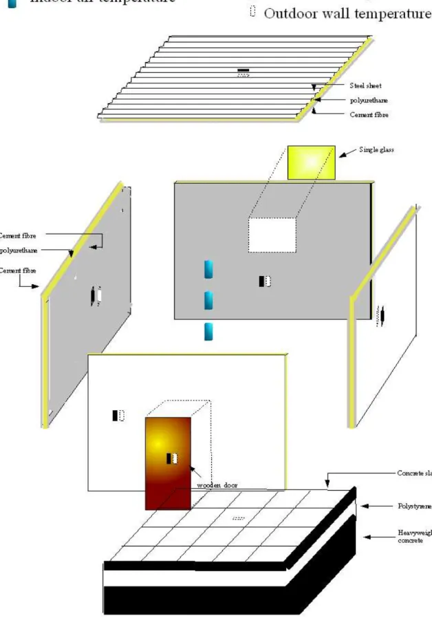
The studied test cell is a 22.50 m³ cubic-shaped building with a single window on the south wall and a door on the north side. All vertical walls are identical and are composed of cement fibre and polyurethane, the roof is constituted of steel, polyurethane and cement fibre and the floor of concrete slabs, polystyrene and concrete (see Fig. 4 for more details concerning the walls constitution). The building under consideration is highly insulated.

The thermal model of the test cell is derived from a lumped approach. A number of assumptions are generally made in order to keep the computational cost of the simulations affordable. The validity of such assumptions will be verified later during the model validation process, when predictions and measurements are compared. The set of assumptions made are enumerated hereafter.

Thermal transfer through walls is deemed unidirectional. Indoor convective heat transfers are represented by the Newton law with a constant exchange coefficient that depends on whether the wall is vertical or horizontal. Short wave indoor radiation is linearized and is also characterized by a constant radiative coefficient. These assumptions seem reasonable when indoor surface temperatures are similar. The indoor air temperature is assumed uniform (this has been confirmed by measurements, given the high insulation of walls, floor and roof). Thermal bridges are neglected and the heat transfer through the floor is also assumed unidirectional with a null flux at the boundaries.

The outdoor convective heat transfer is modelled by a linear relationship proportional to the difference between the surface and outdoor air temperatures. The proportional coefficient (the outdoor convective heat transfer) is a function of the wall or window, wind speed and direction.

Two types of short wave radiations are considered, direct and diffuse solar irradiance on a

(15)

horizontal surface. They are supposed to be absorbed and reflected by walls and also transmitted by the windows. Long-wave heat transfer exchanges are linearized and characterized by a constant radiative heat transfer coefficient. The walls are assumed to interact with the surroundings and the sky. The temperature of the first one is fixed to outdoor air temperature and the fictive sky temperature is either measured or modelled as a function of outdoor air temperature.

The set of equations that governs the energy balance of a building are of the general form :

{

^Y^d^dt^t^T^=G⁼^F^T^T^t^t^^^,U^,^U^t^t^^^,^,^^,^,^t^t^^

where Y is the output vector, T the state vector, U the solicitation vector that perturbs the system, q is a vector of parameters that characterize the building (see Table 1 for a description of the test cell thermal model parameters), e is a vector of unmeasurable stochastic inputs and x is a vector of measurement noise.

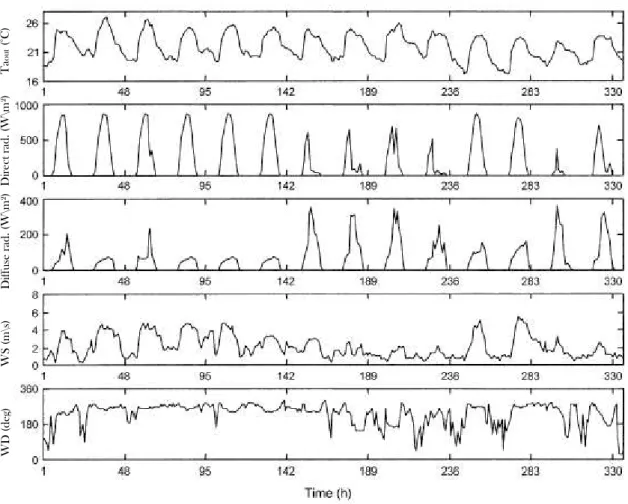
The outdoor solicitations are generally measured or simulated. In the following, they have been measured using a weather station located on the test cell site that recorded every ten seconds outdoor air temperature, relative humidity, global and diffuse solar radiations, wind speed and direction (see Fig. 5). Then, the data, obtained from a 14-day experiment, are under-sampled at one- hour time step. The uncertainty of the measured weather data is neglected in the rest of the paper.

Short wave radiation is not measured but modelled as : Fswr = hr(Tsout – Tsky) where, Fswr is the net short wave flux (W/m²), hr the radiative heat transfer coefficient (W/m²°C), Tsout (°C) the temperature of the outdoor surface and the fictive sky temperature Tsky is set equal to the outdoor dry-air temperature minus a constant parameter K as follows Tsky = Taout – K.

(16)

5.2 Problem 1 : Identification of the most influential walls

A first survey is undertaken to investigate the components (i.e. walls, roof, ground and window) that contribute mostly to the variation of the indoor air temperature. The thermal characteristics of the building are summarized in table 1, by means of the base case values for the parameters. The response of interest is the predicted indoor dry-air temperature, and eigth factors are analyzed: the walls on the four different sides, the window, the door, the roof and the ground. These are analyzed using a two-level full factorial design which assigns two values to each factor: +1 assumes that the component is present with the thermal characteristics defined in table 1 (base values); and -1 assumes that the component is considered perfectly adiabatic, with null indoor and outdoor heat transfer coefficients.

The full factorial design evaluates the model for all possible combinations of factors values. To explore the eight factors, N = 2⁸ model runs are required. Once the simulations are performed, at each time step, the model responses Y_r(t) (r = 1,2, ...,256) are analyzed to compute the hourly polynomial coefficients (see Eq. (3)) from which the hourly ANOVA-based sensitivity indices are obtained. We recall the formulas to estimate the polynomial coefficients:

0t= E[FX]=1

N

∑

r=1 N

Y_rt,

_it= E[x_iFX]=1

N

∑

r=1 N

x_riY_rt , i = 1,2,...8,

ijt= E[x_ix_jFX]=1

N

∑

r=1 N

x_rix_rjY_rt , j>i ...

where xki is the k^th value of xi, the standardized variable, and the bi^t1 ...i^r's are the computed hourly polynomial coefficients at timestep t. Because all the factors combinations are considered, the coefficients so computed are unbiased.

The first-order and total sensitivity indices are plotted in Fig. 6 for the last two days of the simulation (day 13 and 14, when transient effects have disappeared). The ground is the most

(17)

responsible for the variation of indoor air temperature in the nighttime. The ground is also influential, yet to a lesser extent, in the day time together with the door (in the mornings), the roof and the west side wall in the afternoon. The window is relatively involved in the temperature variation but only in the daytime. This is explained by the fact that diffuse solar radiation passing through the window warms up the indoor air. Consequently, its effect decreases quickly at nightfall.

The influence of the window is much higher the 13^th day because it is a cloudy day. The factors contributions are almost additive except at times 298 (10 a.m.) and 305 (5 p.m.). At ten a.m., the door and the window are the most important factors (and they highly interact as their total sensitivity index is much higher than their marginal effect). At five p.m., the dynamics is very complex as the window, the roof and the west wall interact with the ground and the door, while also marginally contributing to the variation of the indoor air temperature.

The importance of the ground is due to the thermal storage capacity of the concrete slabs. Indeed, energy provided by outdoor solicitations are stored by the thermal capacitance of this material in the daytime and released during the night. This fact is confirmed by the analysis of the marginal effect of this factor (see Fig. 7).

At two time points, 10 a.m. and 5 p.m.., there are strong interactions between the factors. This can be explained by change in direction of the heat flux in the test cell. The concrete slabs on the ground start to store energy (10 a.m.) or to release it (5 p.m.). As a consequence, the heat exchange between the ground and the indoor air is almost null putting forward interactions between the walls.

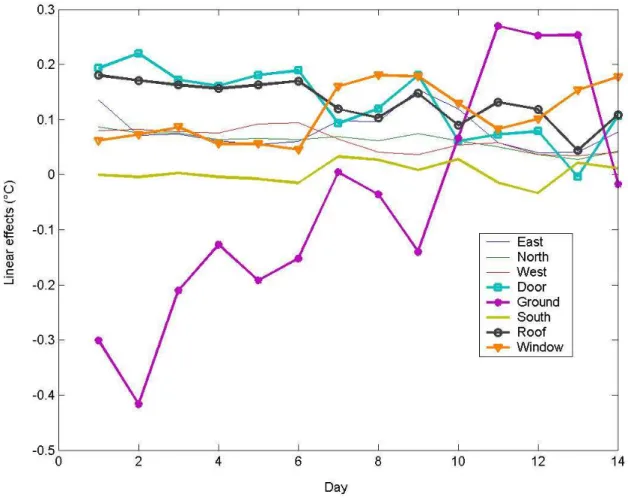
The sensitivity analysis of the daily mean indoor air temperature (Fig. 8) still puts forward the preponderance of the floor, yet it also highlights its thermal inertia on the ten first days of simulation. However, this transient is low (less than 0.4°C). In the rest of the paper, only the four last days of simulations are considered.

(18)

5.3 Problem 2 : Model calibration under uncertainty 5.3.1 The suited model response

The base values for the thermal properties of the material used in the previous section are those found in a former experiment in which the model predictions were fitted to the measurements. But it could be possible that other combinations of parameters make this fit work anyway. Therefore, in this second survey we consider the thermal properties of the materials as affected by uncertainty. To characterize their uncertainty we used the review of existing data-sets of thermo-physical properties of building materials [38], produced by the Building Environmental Performance Analysis Club (BEPAC) in the 90’s. For a given parameter, different values were proposed in this review because of difference in the material conceptions and also because there were no standardized testing procedures for their determination. Parameters that are not reported in the document are assumed uniformly distributed over a generous uncertainty range proposed by one of the authors. The uncertainty ranges are, in some cases, overestimated to ensure that the parameters’ values are plausible.

The choice of the parameters intends to account for different modes of heat transfer. For instance, the density of a material characterizes is thermal mass whereas the thermal conductivity represents the thermal conductance. In the same way, the indoor convective heat transfer coefficient is supposed to account for both indoor convective heat exchange and long-wave radiative heat transfer. The outdoor long-wave heat exchanges modelled by a linear relationship also takes into account heat transfer with the surroundings.

In the approach used here, the generalized likelihood uncertainty estimate (GLUE) [39,40], we aim at identifying the values of the parameters that produce predictions close to empirical measurements. The term close to can be defined either in terms of a likelihood measure Eq. (7) or as a threshold Eq. (8) :

(19)

Y= 1

Lⁿ with L=

∑

t=1 N_obs

T_mt– T_pt ,² or, (7a)

Y=e⁻

L

2 ² (7b)

Y=

{

^{1 if}0 otherwise^∣^T^m^^t^−^T^p^^{t ,}^{∣}^,^∀^t^∈[^1,^N^obs^] (8) with n>0 is a positive integer, Nobs is the number of observations, Tm(t), Tp(t) are respectively the measured and predicted temperature, s², a are given constraint hyperparameters. The two first model responses are continuous whereas the last one is binary. In the next, we use Eq. (7a) with n = 1 as response of interest, given that the choice of the output impacts on the sensitivity indices and not on the conclusion of the analysis.

5.3.2 Results and discussion

A LHS sample matrix of size N = 500 has been generated and propagated through the test cell thermal model. For each trial, the predicted indoor air and surfaces temperatures as well as the outdoor surfaces temperatures were saved for a total of 10 model outputs. The computation lasted 52 minutes on a 1.30 GHz processor computer for 14 days hourly simulations. Then, the likelihood measures were computed and the first-order sensitivity indices estimated using Eq. (4) (the order M of the polynomial was set to 4).

We decided that, for a given model output, if a parameter has sensitivity index below 5% for the ten likelihood measures, then the parameter is non significant. We found that ten parameters are responsible for the goodness of fit between the model predictions and the measurements. They are listed in table 2 as well as their sensitivities. Note that the model is non additive

0.35≤

∑

i=1

35 S_i≤0.78 with respect to all the 10 model outputs. This is a consequence of the model

overparametrization, well-known in inverse problems, and termed as equifinality by Beven [41]. In

(20)

other words, different combinations of parameters values can yield the same predictions.

Consequently, modellers can hardly find one single set of parameters to reproduce the system behaviour. Instead, they will find a set of parameters combinations that result from a conjoint probability density function with a complex correlation structure (see [42] for a simple illustration).

To check whether the remaining twenty-five parameters are not involved in the good behaviour of the model, the total sensitivity indices of the group Xg1 = {X14,X15,X16,X24,X26,X27,X28,X29,X30,X34} are computed. To this purpose, the factors set are split into two groups. Then, an input sample of size 500 has been generated by only modifying the factors values of Xg1 according to the scheme of Fig. 3. Then, the total sensitivity index of the group has been estimated (with Eq. (5)). Table 2 shows that the former is closed to unity regardless of the output confirming that Xg¹ contains the inputs that are mostly responsible of the variation of the likelihoods. These parameters are referred to as behavioral. Among these the most important is X16 (i.e. absorptivity of outdoor surfaces). This indicates that the uncertainty of the outdoor absorptivity should be reduced or the radiation processor improved or that better measurements of solar irradiance should be obtained.

[Insert Table 1 about here]

[Insert Table 2 about here]

The model is capable to simulate the underlying phenomenon if the input values can produce model responses in a small range that contains the measurements. For each output, we estimate the smallest relative uncertainty bound for which the model is able to provide responses that remain inside the bound at each timestep. The results show that the model is able to predict indoor air temperatures accurately (the highest discrepancy is lower than 5%, refer to table 2 and figures 9-10) but performs worse as far as outdoor surface temperature of the roof are concerned (i.e., the smallest relative uncertainty bounds is 29%). In particular, the model is unable to describe the heat transfers upon the roof and it fails to reproduce the entire thermal behaviour of the test cell. SA results

(21)

indicate that the way convective and solar radiation heat transfers are accounted for in the model for the roof should be revised.

Results of the previous application (see section 5.3.1) have highlighted the preponderance of the thermal mass of the ground and the heat transfers through the window and the door on indoor air temperature. The good performance of the model for indoor temperatures prediction means that the former is able to reproduce the thermal mass of the slabs as well as the heat transfer by conduction through the door and the amount of diffuse solar radiation passing through the window.

5.3.3 Further improvements of the model

The previous analysis highlighted that the model predicts the outdoor surface temperature of the roof with poor accuracy and that, for this response, the parameters involved in the modelling of outdoor convective heat transfer coefficient are preponderant. So, the former has been modified as follows (for all outdoor surfaces) :

hci = ai|DT|ⁿⁱ + biV^cⁱ (instead of hci = ai + biV^cⁱ)

where the term DT = (Taout-Tsout) is introduced to account for the variability of natural convection.

The exponent n is an additional uncertain input labeled X36 with uncertainty range set to [0,2]. The uncertainty range of {X22,X25,X28,X31} is set to [0,10] as compared to the previous analysis (see table 1). The uncertainty ranges of the ai's have been reduced in order to ensure that the values of the outdoor convective heat transfer coefficient vary in a plausible range. Indeed, |DT| reach 10°C for some surfaces. A new SA based on a LHS sample of size 500 has been generated and executed for all model outputs. The same inputs as in the previous analysis are identified as important as well as the new input X36 for the roof temperature. The main interesting result is an improvement of the

(22)

model response for outdoor surface temperature of the roof without modifying the accuracy of the other responses (see the last row of table 1). Indeed, the model is now able to predict the output in the 15% uncertainty bounds of measurements.

Conclusion

We encourage modellers to perform sensitivity analysis during the phase of model building, and developers of thermal models for edifices in particular. Indeed, they can get better insight on the model at hand, understanding the relationships that link inputs and predictions. This can in turn help to identify weak parts of the model when predictions are tested again available measurements. In section 4, two methods to estimate first-order sensitivity measures are described: the one using generalized additive models and that of Sobol'. This latter method is also available in the SimLab package [24].

In a case study proposed in the paper, the calibration of the model is undertaken using thirty five parameters and ten outputs. In the multi-output calibration adopted here different inputs are simultaneously activated that have an effect on the various outputs. The sensitivity analysis pointed out the few active model inputs and the interactions that produce predictions close to measurements.

Although the model was able to predict the indoor temperatures rather accurately, sensitivity analysis was helpful in showing that the model was unable to provide satisfactory outcomes for outdoor surfaces temperatures and that outdoor convective heat transfers had to be modelled better.

Additional improvements in the model can be done by further exploiting sensitivity analysis results.

(23)

References

[1] Fürbringer J.M., Roulet C.A., Comparison and Combination of Factorial and Monte Carlo Design in Sensitivity Analysis, Building and Environment, Vol.30, pp.505-519, 1995.

[2] De Witt M.S., Identification of the Important Parameters in Thermal Building Simulation, Journal of Statistical Computation and Simulation, Vol.57, pp.305-320, 1997.

[3] Rahni N., Ramdani N., Candau Y., G. Guyon, Application of Group Screening to Dynamic Building Energy Simulation Models, Journal of Statistical Computation and Simulation, Vol.57, pp.285-304, 1997.

[4] Mara T.A., Rakoto Joseph O., Comparison of some Efficient Methods to Evaluate the Main Effect of Computer Model Factors, Journal of Statistical Computation and Simulation, Vol.78, pp.167-178, 2008.

[5] Aude P., Béghein C., Depecker P., Inard C., Perturbation of the Input Data of Models Used for the Prediction of Turbulent airflow in an Enclosure, Numerical Heat Transfer, Vol.34, pp.139-164, 1998.

[6] Palomo del Barrio E., Guyon G., Theoretical Basis for Empirical Model Validation using Parameters Space Analysis Tools, Energy and Buildings, Vol.35, pp.985-996, 2003.

[7] Mara T.A., Boyer H., Garde F., Parametric Senstivity Analysis of a Test Cell Thermal Model Using Spectral Analysis, Journal of Solar Energy Engineering, Vol.124, pp.237-242, 2002.

[8] Saltelli A., Ratto M., Tarantola S., Campolongo F., Sensitivity Analysis Practices : Strategies for Model-Based Inference, Reliability and System Safety, Vol.91, pp.1109-1125, 2006.

[9] Saltelli A., Tarantola S., On the Relative Importance of Input Factors in Mathematical Models : Safety Assessment for Nuclear Waste Disposal, Journal of the American Statistical Association, Vol.97, pp.702-709, 2002.

(24)

[10] Saltelli A.,Tarantola S., Campolongo F., Ratto M., Sensitivity Analysis in Practice, John Wiley, 2004.

[11] Morris M.D., Factorial Sampling Plans for Premilinary Computational Experiments, Technometrics, Vol.33, pp.161-174, 1991.

[12] Campolongo F., Cariboni J., Saltelli A., An Effective Screening Design for Sensitivity Analysis of Large Models, Environmental Modelling & Software, Vol.22, pp.1509-1518, 2007.

[13] Sobol I.M., Sensitivity Analysis for Non Linear Mathematical Models, Math. Modelling and Computatonial Experiment, Vol.1, pp.407-414, 1993.

[14] Borgonovo E., A New Uncertainty Importance Measure, Reliability and System Safety, Vol.92, pp.771-784, 2007.

[15] Borgonovo E. & Tarantola S., Moment Independent And Variance-Based Sensitivity With Correlations: An Application to the Stability of a Chemical Reaction, International Journal of Chemical Kinetics, Vol., pp., 2008.

[16] Saltelli A., Making Best Use of Model Evaluations to Compute Sensitivity Indices, Computer Physics Communication, Vol.145, pp.280-297, 2002.

[17] Saltelli A., Tarantola S., Chan K., A Quantitative Model-Independent Method for GSA of Model Output, Technometrics, Vol.41, pp.39-56, 1999.

[18] Rabitz H., Alis O., Shorter J. Shim K., Efficient Input-Output Model Representations, Computer Physics Communication, Vol.117, pp.11-20, 1999.

[19] Morris M., Moore L.M., MacKay M.D., Sampling Plans Based on Balanced Incomplete Block Designs for Evaluating the Importance of Computer Model Inputs, J. Statistical Planning and Inferences, Vol.136, pp.3203-3220, 2006.

[20] Oakley J.E., O'Hagan A., Probabilistic Sensitivity Analysis of Complex Models : A Bayesian Approach, Journal of Royal Statistical Society (B), Vol.66, pp.751-769, 2004.

[21] Sudret B., Global Senstivity Analysis Using Polynomial Chaos Expansions, Reliability and System Safety, Vol.93, pp.964-979, 2008.

(25)

[22] Tarantola S., Gatelli D, Mara T.A., Random Balance Designs for the Estimation of First-order Sensitivity Indices, Reliability and System Safety, Vol.91, pp.717-727, 2007.

[23] Fürbringer J.M., Roulet C.A., Confidence of Simulation Results : Put a SAM in Your Model, Energy & Buildings, Vol.30, pp.61-71, 1999.

[24] SIMLAB, Simulation environment for uncertainty and sensitivity analysis., Version 3.1 Joint Research Centre of the European Commission, available at http://jrc.simlab.ec.europa.eu, 2007.

[25] De Rocquigny E., Devictor N., Tarantola S., Uncertainty in Industrial Practice: A Guide to Quantitative Uncertainty Man, John Wiley, 2008.

[26] Fisher R.A., The Design of experiment, HAFNER press, 1935.

[27] Satterthwaite F.E., Random Balance Experimentation, Technometrics, Vol.1, pp.111-138, 1959.

[28] Box G.E.P., Hunter W.G., Hunter J.S., Statistics for Experimentaters, John Wiley, 1978.

[29] Andres T.H., Sampling Method and Sensitvity Analysis for Large Parameters Sets, Journal of Statistical Computation and Simulation, Vol.16, pp.97-110, 1997.

[30] Bettonvil B., Kleijnen J.P.C, Searching for Important Factors in Simulation Models with Many Factors : Sequential Bifurcation, European J. of Operational Research, Vol.96, pp.180-194, 1997.

[31] Helton J.C., Jonhson J.D., Sallaberry C.J., Storlie C.B., Sensitivity Analysis of Model Output:

SAMO 2004, Reliability Engineering and System Safety, Vol.91, pp.1175-1209, 2006.

[32] Iman R.I., Conover W.J., A Distribution-Free Approach to Inducing Rank Correlation Among Input Variables, Communications in Statistics : Simulation and Comp, Vol.B11, pp.311-334, 1982.

[33] Sallaberry C.J., Helton J.C., Extension of Latin Hypercube Samples with Correlated Variables, Reliability Engineering and System Safety, Vol.93, pp.1047-1059, 2008.

[34] HastieT.J., Tibshirani R.J., Generalized Additive Models, Chapman & Hall, 1990.

[35] Sobol I.M., Tarantola S., Gatelli D., Kucherenko S.S., Mauntz W., Estimating the Approximation Error when Fixing Unessential Factors in GSA, Reliability and System Safety,

(26)

[36] Mara T.A., Garde F., Boyer H., Mamode M., Empirical Validation of the Thermal Model of a Passive Solar Cell Test, Energy & Buildings, Vol.33, pp.589-599, 2000.

[37] Mara T.A., Fock E., Garde F., Lucas F., Development of a new Model of Single-Speed Air Conditioners at Part-Load Conditions for Hourly Simulations, Journal of Solar Energy Engineering, Vol.127, pp.294-301, 2005.

[38] Clarke J.A., Yaneske P.P., Pinney A.A., The Harmonisation of Thermal Properties of Building Materials, BEPAC,1991.

[39] Hornberger G.M. and Spear R.C., An Approach to the Preliminary Analysis of Environmental Systems, Journal of Environmental Management, Vol.12, pp.7-18, 1981.

[40] Spear R.C., Grieb T.M., Shang N., Parameter Uncertainty and Interaction in Complex Environmental Models, Water Resources Research, Vol.30, pp.3159-3169, 1994.

[41] Beven K., A Manifesto for the Equifinality Thesis, Journal of Hydrology, Vol.320, pp.18-36, 2006.

[42] Ratto M., Tarantola S., Saltelli A., Sensitivity Analysis in Model Calibration : GSA-GLUE Approach, Computer Physics Communication, Vol.136, pp.212-224, 2001.

(27)

List of Figures

Fig. 1 : Example of latin hypercube sampling for two independent random variables X1 and X2.

The probability distribution of X1 is N(0,1) and of X2 is U(-1,1). On the left, is plotted the cumulative distribution of the normal distribution and it is shown how the uncertainty range is divided into five contiguous intervals of equal probability. On the right, are plotted the sampled points in the factors space.

Fig. 2 : Uncertainty representations of a random variable. The density distribution represented by the histogram on the left gives the most probable value of the variable. With the cumulative distribution (on the right) one can determine the uncertainty range for different quantiles.

Fig. 3 : Sobol' sampling strategies to compute the global sentivity indices of individual input factors or groups of factors. X(r) is a sample matrix of N rows and p columns. Each row is a set of input factors value and each column is a vector of values assigned to the factor. X(r)ki is the kth value of Xi in the rth sample matrix.

Fig. 4 : Scheme of the thermal test cell, its constitution and instrumentation.

Fig. 5 : The hourly weather data during the fourteen days of experimentation.

Fig. 6 : Hourly influence of the test cell's surface on indoor air temperature. The most influence one is the ground. It is particularly preponderant in the nighttime and less influent during the day. At times 298 and 305 (10hr and 17hr) its marginal influence is null but its interactions with the other components are not negligible. Interactions at any other timestep are less important.

Fig. 7 : Hourly linear effects of the test cell components. The thermal capacitance of the ground is particularly highlighted. The concrete slabs absorb energy in the daytime and release it in the nighttime. This explains its negative effect in the daytime and positive effect during the night. The linear effect of the other components appears in the daytime and almost negligible in the nighttime as confirmed by the global sensitivity indices.

Fig. 8 : Daily linear effects of the test cell components on the indoor air temperature. The thermal mass of the ground slightly perturbs the predictions at the beginning of the simulation.

Fig. 9 : The best predicted indoor air temperatures belong to the 3.5% interval bounds of measurements.

Fig. 10 : The best predicted outdoor surface temperatures of the roof belong to the 29% interval bounds of measurements. The initial model is not accurate. The problem occurs in the nighttime of the second day (around time 265).

(28)

-3 -2 -1 0 1 2 3 0

0.1 0.2 0.3 0.4 0.5 0.6 0.7 0.8 0.9 1

%

X_i

-1.25 -0.45 0.05 0.6 2

-3 -2 -1 0 1 2 3

0 0.1 0.2 0.3 0.4 0.5 0.6 0.7 0.8 0.9 1

%

X_i

-1.25 -0.45 0.05 0.6 2

-3 -2 -1 0 1 2 3

-1 -0.8 -0.6 -0.4 -0.2 0 0.2 0.4 0.6 0.8 1

X1 X2

+ +

+

+ +

+ ++ +

++ +

+ +

+ ++

+ +

++ +

++ + +

++

+ +

+

-3 -2 -1 0 1 2 3

-1 -0.8 -0.6 -0.4 -0.2 0 0.2 0.4 0.6 0.8 1

X1 X2

-3 -2 -1 0 1 2 3

-1 -0.8 -0.6 -0.4 -0.2 0 0.2 0.4 0.6 0.8 1

X1 X2

+ +

+

+ +

+ ++ +

++ +

+ +

+ ++

+ +

++ +

++ + +

++

+ +

+

+ +

+

+ +

+ ++ +

++ +

+ +

+ ++

+ +

++ +

++ + +

++

+ +

+

Fig. 1 : Example of latin hypercube sampling for two independent random variables X1 and X2. The probability distribution of X1 is N(0,1) and of X2 is U(-1,1). On the left, is plotted the cumulative distribution of the normal distribution and it is shown how the uncertainty range is divided into five contiguous intervals of equal probability. On the right, are plotted the sampled points in the factors space.

(29)

23 24 25 26 27 28 29 30 31 32 0

0.1 0.2 0.3 0.4 0.5 0.6 0.7 0.8 0.9 1

Y 0.975

0.025

Intervalle d'incertitude sur Y à 95%

22 24 26 28 30 32 34

0 20 40 60 80 100 120 140 160

Y

Fig. 2 : Uncertainty representations of a random variable. The density distribution represented by the histogram on the left gives the most probable value of the variable. With the cumulative distribution (on the right) one can determine the uncertainty range for different quantiles.

95% confidence interval

The most probable value of Y