Parameter Estimation, Sensitivity Analysis and Optimal Control of a Periodic Epidemic Model with Application to HRSV in Florida

Published online in International Academic Press (www.IAPress.org)

Parameter Estimation, Sensitivity Analysis and Optimal Control

of a Periodic Epidemic Model with Application to HRSV in Florida

Silv´erio Rosa

, Delfim F. M. Torres

1_{Department of Mathematics and Instituto de Telecomunicac¸˜oes (IT),}

University of Beira Interior, 6201-001 Covilh˜a, Portugal.

2_{Center for Research and Development in Mathematics and Applications (CIDMA),}

Department of Mathematics, University of Aveiro, 3810-193 Aveiro, Portugal.

Abstract A state wide Human Respiratory Syncytial Virus (HRSV) surveillance system was implemented in Florida in 1999 to support clinical decision-making for prophylaxis of premature infants. The research presented in this paper addresses the problem of fitting real data collected by the Florida HRSV surveillance system by using a periodic SEIRS mathematical model. A sensitivity and cost-effectiveness analysis of the model is done and an optimal control problem is formulated and solved with treatment as the control variable.

Keywords Human Respiratory Syncytial Virus (HRSV), Compartmental Mathematical Models, Estimation of Parameters, Optimal Control

AMS 2010 subject classifications34C60, 49M05, 92D30 DOI:10.19139/soic.v6i1.472

1. Introduction

Human respiratory syncytial virus (HRSV) is a virus that causes respiratory tract infections. It is a major cause of lower respiratory tract infections and hospital visits during infancy and childhood. A prophylactic medication, palivizumab, can be employed to prevent HRSV in preterm infants (under 35 weeks gestation), infants with certain congenital heart defects or bronchopulmonary dysplasia, and infants with congenital malformations of the airway. Treatment is limited to supportive care, including oxygen therapy. In temperate climates, there is an annual epidemic during the winter months. In tropical climates, infection is most common during the rainy season. In the United States, 60% of infants are infected during their first HRSV season, and nearly all children will have been infected with the virus by two to three years of age [9]. Of those infected with HRSV, 2 to 3% will develop bronchiolitis, necessitating hospitalization [10]. Natural infection with HRSV induces protective immunity, which wanes over time, possibly more so than other respiratory viral infections, and thus people can be infected multiple times. Sometimes an infant can become symptomatically infected more than once, even within a single HRSV season. Severe HRSV infections have increasingly been found among elderly patients. Young adults can be re-infected every five to seven years, with symptoms looking like a sinus infection or a cold. The Florida Department of Health provides an integrated and reliable HRSV system, with data from hospitals and laboratories [8].

Mathematical models can project how infectious diseases progress, to show the likely outcome of an epidemic, and help inform public health interventions. In epidemiology, compartmental models serve as the base mathematical framework for understanding the complex dynamics of these systems. Such compartments, in the

∗_{Correspondence to: Delfim F. M. Torres (Email: delfim@ua.pt). Department of Mathematics, University of Aveiro, 3810-193 Aveiro,}

Portugal.

simplest case, stratify the population into two health states: susceptible to the infection of the pathogen, often denoted byS, and infected by the pathogen, often denoted by the symbolI. The way that these compartments interact is based upon phenomenological assumptions, and the model is built up from there. These models are usually investigated through ordinary differential equations. To push these basic models to further realism, other compartments are often included, most notably the recovered/removed/immune compartment, often denoted byR. A crucial question consists to find parameters for the particular disease under study, and use those parameters to calculate the effects of possible control interventions, like treatment or vaccination. Then the central issue is how to implement such interventions in an optimal way. This investigation program has been recently carried out for several infectious diseases, as diverse as dengue [5,23], tuberculosis [6,25], Ebola [11,21], HIV/AIDS [26,27], and cholera [12,15]. Here we investigate such approach to HRSV.

A comparison of the standard SIRS model with a more complex model of HRSV transmission, in which individuals acquire immunity gradually after repeated exposure to infection, is given in [30]. In [1], an age-structured mathematical model for HRSV is proposed, where children younger than one year old, who are the most affected by this illness, are specially considered. Real data of hospitalized children in the Spanish region of Valencia is used in order to determine some seasonal parameters of the model [1]. A numerical scheme for the SIRS seasonal epidemiological model of HRSV transmission is proposed in [3]. It turns out that solutions for HRSV compartmental models are typically periodic [2]. For this reason, in this work we propose the use of optimal control theory to a non-autonomous SEIRS model [13] and show its usefulness in agreement with real HRSV data provided by the Florida Department of Health [8].

The paper is organized as follows. In Section2, we briefly review the SIRS and SEIRS epidemic models. Our results are then given in Section3: parameter estimation of the SEIRS model with real data of Florida (Section3.1); sensitivity analysis (Section3.2); and optimal control and numerical simulations (Sections3.3and 3.4). We end with Section4of conclusions and some future perspectives.

2. Review of some recent HRSV mathematical models

We focus on compartmental models that divide the population into mutually exclusive distinct groups (of susceptible, or infected, or immune individuals, or . . . ) and we use deterministic continuous transitions between those groups, also known as states. Due to the seasonality of HRSV, the models that best fit real data are periodic and, therefore, non-autonomous. In [30], two models are proposed where the transmission is periodic: (i) a simple model with only three compartments, known as SIRS (Section2.1); (ii) and a more complex model with seventeen compartments, named MSEIRS4. However, it is shown that the simpler model is closer to real data [30]. Zang et al. [31] use a non-autonomous SEIR model where, beyond the periodicity in the transmission rate, the annual recruitment rate is also periodic. This assumption is due to opening and closing of schools [31]. Here we adopt such ideas and consider a simple non-autonomous and periodic SEIRS model (Section2.2).

2.1. SIRS model

In the SIRS model, one considers that the population consists of susceptible (S), infected and infectious (I), and recovered (R) individuals. A characteristic feature of HRSV is that immunity after infection is temporary, so that the recovered individuals become susceptible again [30]. The model depends on several parameters: parameterµ, which denotes the birth rate, assumed equal to the mortality rate;γ, which is the rate of immunity loss; andν, which is the rate of loss of infectiousness. Moreover, the influence of the seasonality on the transmission parameterβ is modeled by the cosine function. Precisely, and using the linear mass action law [30], the SIRS model for HRSV is given by the following system of ordinary differential equations [30]:

     ˙ S(t) = µ− µS(t) − β(t)S(t)I(t) + γR(t), ˙

I(t) = β(t)S(t)I(t)− νI(t) − µI(t),

˙

R(t) = νI(t)− µR(t) − γR(t),

where β(t) = b0(1 + b1cos(2πt + Φ)). Note that b0 is the average of the transmission parameter β, b1 is the amplitude of the seasonal fluctuation in the transmission parameterβ, while Φis an angle that will be chosen later in agreement with the real data forI(t).

2.2. SEIRS model

In order to incorporate some important features of HRSV into the model while keeping it simple, we extend the model (1) of Section2.1by using the ideas in [13]: firstly, we include a latency period by introducing a groupEof individuals who have been infected but are not yet infectious, these individuals becoming infectious at a rateεand the latency period being equal to the time between infection and the first symptoms; secondly, and similar to [31], we consider that the annual recruitment rate is seasonal due to schools opening/closing periods. The equations of the SEIRS model are then given by

         ˙ S(t) = λ(t)− µS(t) − β(t)S(t)I(t) + γR(t), ˙

E(t) = β(t)S(t)I(t)− µE(t) − εE(t),

˙

I(t) = εE(t)− µI(t) − νI(t),

˙

R(t) = νI(t)− µR(t) − γR(t),

(2)

whereλ(t) = µ(1 + c1cos(2πt + Φ))is the recruitment rate, including newborns, immigrants, etc. Parameterc1is the amplitude of the seasonal fluctuation in the recruitment parameterλandΦan angle to be conveniently chosen.

3. Main results

We begin by investigating how realistic the models discussed in Section2are with respect to HRSV and real data from Florida [8]. For that we need a proper estimation of the parameter values.

3.1. Parameter estimation

During model fitting, the values of the parametersµ(birth rate),ε(infectious rate),ν (rate of infectiousness loss) and γ (rate of immunity loss) were held constant. See Table1, where we usento denote the average number of monthly HRSV cases reported. The values ofε,ν andγwere taken from [30]. For the birth rate,µ, we used the value given in [7] for the state of Florida. In agreement with Section2.1, we have set the birth rate equal to the mortality rate, so that one obtains a constant population during the period under study. This simplification is justified when, as in this case, the annual infection rate is much bigger than the growth of population. To simplify analysis, we set the total population equal to one and use fractions for the values of state variables. Values of four parameters were determined by fitting the model: (i) the mean of the transmission parameter, b0; (ii) its relative seasonal amplitude,b1; (iii) the angleΦ; and (iv) a scaling factors, which scales the number of infectious individuals to the empirical case reported in our unit scaled model. The angleΦwas normalized in the following way: for a value of zero, a maximum of the cosine function used inβ(t)(and also used inλ(t)) coincides with the first maximum of the empirical cases. The models were fitted to data on the reported number of positive tests of HRSV disease, per month, in the State of Florida, excluding North region, between September 2011 and July 2014 (35 months). The data was obtained from the Florida Department of Health [8]. Our results are given in Figure1.

Table 1. Results of model fitting.

model µ ν γ ε b0 b1 c1 s Φ n R0

SIRS 0.0113 36 1.8 – 74.2 0.14 – 35000 7π/5 932 2.06 SEIRS 0.0113 36 1.8 91 88.25 0.17 0.17 35000 7π/5 932 2.45

time

Sep 2011 Feb 2012 Aug 2012 Feb 2013 Aug 2013 Feb 2014 Jul 2014 0 500 1000 1500 2000 2500 Florida Empiric SEIRS SIRS

Figure 1. Comparison of the number of infective individuals registered in the state of Florida [8] with the ones predicted by models SIRS (1) and SEIRS (2) with the parameter values of Table1.

predictive cases of HRSV infection given by models (1) and (2). Leterepresent the relative error, computed by

e = ∥Imodel− Iempiric∥2 ∥Iempiric∥2

,

whereI_empiricis the real data obtained from [8] andI_modelthe one predicted by the SIRS or SEIRS models. The results shown in Figure1correspond to a relative error of 0.066% and 0.060% of infants per year with respect to the total child population of Florida in 2014, excluding North region, respectively for SIRS or SEIRS models. We note that the values ofµ,ν,γandεare annual rates. The difference between the two models, in terms of absolute errors, clearly justifies SEIRS’ superiority.

3.2. Sensitivity analysis

One of the most important thresholds while studying infectious disease models is the basic reproduction number [29]. The basic reproduction number of the SIRS model was computed in [30]. Assuming that the transmission and the recruitment parameters are constant, the basic reproduction number for the SEIRS model is given by (see [16])

R0=

βε

(µ + ν)(ε + µ). (3)

Now we do a sensitivity analysis for the basic reproduction number (3). Such analysis tells us how important each parameter is to disease transmission. This information is crucial not only for experimental design, but also to data assimilation and reduction of complex nonlinear models [20]. Sensitivity analysis is commonly used to determine the robustness of model predictions to parameter values, since there are usually errors in data collection and presumed parameter values. It is used to discover parameters that have a high impact onR0 and should be targeted by intervention strategies. More precisely, sensitivity indices’s allows to measure the relative change in a variable when parameter changes. For that we use the normalized forward sensitivity index of a variable, with respect to a given parameter, which is defined as the ratio of the relative change in the variable to the relative change in the parameter. If such variable is differentiable with respect to the parameter, then the sensitivity index is defined using partial derivatives, as follows (see [4,22]).

Definition 1

The normalized forward sensitivity index of R0, which is differentiable with respect to a given parameterp, is defined by ΥR0 p = ∂R0 ∂p p R0 .

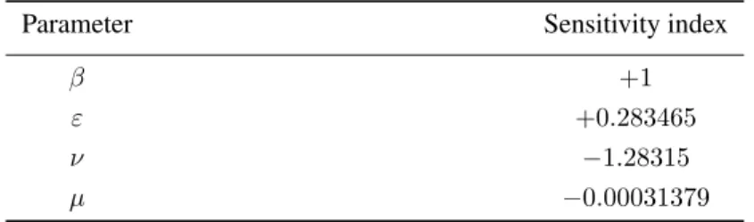
One can easily compute an analytical expression for the sensitivity ofR0, using the explicit formula (3), to each parameter that it includes. The values of the sensitivity indices for the parameters values of Table1 are presented in Table2. Note that the sensitivity index may depend on several parameters of the system, but also can be constant, independent of any parameter. For example,ΥR0

β = +1, meaning that increasing (decreasing)βby a given percentage increases (decreases) alwaysR0by that same percentage. The estimation of a sensitive parameter

Table 2. Sensitivity ofR0evaluated for the parameter values given in Table1, according with (3) and Definition1.

Parameter Sensitivity index

β +1

ε +0.283465

ν −1.28315

µ −0.00031379

should be carefully done, since a small perturbation in such parameter leads to relevant quantitative changes. On the other hand, the estimation of a parameter with a small value for the sensitivity index does not require as much attention to estimate, because a small perturbation in that parameter leads to small changes [14]. According with Table2, we should pay special attention to the estimation of parametersν,b0(mean value ofβ(t)) andε. In contrast, the estimation of the rate of birth,µ, (or rate of mortality) does not require as much attention because of its low value of the sensitivity index. This is well illustrated in Figure2, where we can see in Figure2athe graphics of the number of infectives with and without an increment of 10% for the parameterν(most sensitive parameter), and in Figure2bfor parameterµ(less sensitive parameter).

time

Sep 2011 Feb 2012 Aug 2012 Feb 2013 Aug 2013 Feb 2014 Jul 2014 0 500 1000 1500 2000 Original ν Increased ν

(a) Impact of the variation ofνin the number of infectives I.

time

Sep 2011 Feb 2012 Aug 2012 Feb 2013 Aug 2013 Feb 2014 Jul 2014 0 500 1000 1500 2000 Original µ Increased µ

(b) Impact of the variation of µ in the number of infectivesI(difference not visible).

Figure 2. Infected number of individuals predicted by SEIRS model with original parameter values as in Table1and with an increase of 10% of a specific parameter:νin (a) andµin (b).

3.3. Optimal control

To investigate some optimal control measures, we choose the SEIRS model, which provides a better fitting of available real data, as shown in Section3.1. The evolution on the number of susceptible, exposed, infective and recovered, depend on some factors that can be controlled. In case of HRSV, treatment is the most realistic. For this reason, we consider the following optimal control problem:

         ˙ S(t) = λ(t)− µS(t) − β(t)S(t)I(t) + γR(t), ˙

E(t) = β(t)S(t)I(t)− µE(t) − εE(t),

˙

I(t) = εE(t)− µI(t) − νI(t) − T(t)I(t),

˙

R(t) = νI(t)− µR(t) − γR(t) + T(t)I(t),

(4)

subject to given initial conditions

S(0), E(0), I(0), R(0)>0, (5)

whereTdenotes treatment (Tis the control variable). Note that in the absence of control measures, that is, when T(t) ≡ 0, system (4) reduces to (2). We consider the set of admissible control functions

Ω ={T(·) ∈ L∞(0, tf) : 06T(t)6Tmax,∀t ∈ [0, tf]} .

Our purpose is to minimize the number of infectious individuals and the cost required to control the disease by treating the infected. Precisely, the optimal control problem consists in

min J (I, T) = ∫ tf 0 ( κ1I(t) + κ2T2(t) ) dt subject toS(t) = λ(t)˙ − µS(t) − β(t)S(t)I(t) + γR(t) ˙

E(t) = β(t)S(t)I(t)− µE(t) − εE(t)

˙

I(t) = εE(t)− µI(t) − νI(t) − T(t)I(t)

˙

R(t) = νI(t)− µR(t) − γR(t) + T(t)I(t)

(6)

with 0 < κ1, κ2<∞. To solve the problem, we apply the celebrated Pontryagin maximum principle [19]: the Hamiltonian is given by

H = κ1I + κ2T2+ p1(λ− µS − βSI + γR) + p2(βSI− µE − εE)

+ p3(εE− µI − νI − TI) + p4(νI− µR − γR + TI);

the maximality condition ensures that the extremal control is given by T(t) = min { max { 0,(p3(t)− p4(t))I(t) 2κ2 } ,Tmax } ; (7)

while the adjoint system asserts that the co-state variablespi(t),1≤ i ≤ 4, satisfy relations

˙ p1=− ∂H ∂S ⇔ ˙p1= p1(µ + β(t)I)− β(t)Ip2, ˙ p2=− ∂H ∂E ⇔ ˙p2= p2(µ + ε)− εp3, ˙ p3=− ∂H ∂I ⇔ ˙p3=−κ1+ β(t)p1S− p2β(t)S + p3(µ + ν +T) − p4(ν +T), ˙ p4=− ∂H ∂R ⇔ ˙p4=−γp1+ p4(µ + γ) (8)

and transversality conditions

p1(tf) = p2(tf) = p3(tf) = p4(tf) = 0. (9) Therefore, in order to solve the optimal control problem (6), we solve the following boundary value problem:

                                       ˙ S =λ(t)− µS − β(t)SI + γR ˙

E =β(t)SI− µE − εE

˙

I =εE− µI − νI − TI

˙ R =νI− µR − γR + TI ˙ p1=p1(µ + β(t)I)− β(t)Ip2 ˙ p2=p2(µ + ε)− εp3 ˙ p3=− κ1+ β(t)p1S− p2β(t)S + p3(µ + ν +T) − p4(ν +T) ˙ p4=− γp1+ p4(µ + γ) (10)

with given initial conditions

S(0) = s0, E(0) = e0, I(0) = i0, R(0) = r0

and transversality conditions (9), whereT(t)is given by (7). This is done numerically in Section3.4. 3.4. Numerical results and cost-effectiveness analysis for the optimal control model

Two algorithms were implemented to obtain and confirm the numerical results. One approach solves the optimal control problem numerically using a fourth order Runge–Kutta iterative method. First we solve the system (4) with initial conditions for the state variables and a guess for the control over the time interval[0, tf], by the forward Runge–Kutta fourth order procedure, and obtain the values of the state variables S, E,I and R. Using those values, then we solve the system (8) with the transversality conditions (9), by the backward fourth order Runge– Kutta procedure, and obtain the values of the co-state variables. The control is updated by a convex combination of the previous control and the value from (7). The iteration is stopped when the values of the unknowns at the earlier iteration are very close to the ones at the current iteration. The results coincide with the ones obtained by a similar iterative method that, in each iteration, solves the boundary value problem (10) using the MATLABbvp4c routine.

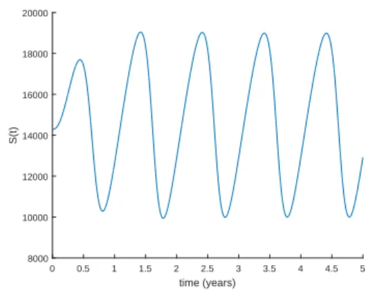
In what follows, we consider that, for simplicity, Tmax= 1 and the other parameters are fixed according to Table1, with exception to the angleΦthat is assumed to beπ/2. Such value allows that the transmission parameter initial value be the average,β(0) = b0, and the recruitment rate initial value also be the average,λ(0) = µ. The initial conditions, given by Table3, are obtained as the nontrivial equilibria for the system (4) with no control, corresponding to the population state prior the introduction of the treatment. We also assume thattf = 5because the World Health Organization goals for most diseases are usually fixed for 5 years periods.

Table 3. Initial conditions for the optimal control problem with parameters given by Table1, excepting angleΦ that is assumed to beπ/2. The values correspond to the endemic equilibrium of (4) before the introduction of treatment.

sS(0) sE(0) sI(0) sR(0)

14284 385 974 19357

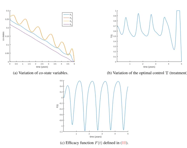
The solution for the optimal control problem is illustrated in Figures3,4aand4b. The periodic nature of the disease influences the evolution of the four state variables. We can also see that the control is a continuous function that shows some nonregularity at the end of the time interval[0, tf]. This behaviour is explained by the irregular oscillation of the co-state variables, on which the control depends.

time (years) 0 0.5 1 1.5 2 2.5 3 3.5 4 4.5 5 S(t) 8000 10000 12000 14000 16000 18000 20000

(a) Evolution of the number of susceptible individuals.

time (years) 0 0.5 1 1.5 2 2.5 3 3.5 4 4.5 5 E(t) 100 200 300 400 500 600 700 800 900

(b) Evolution of the number of exposed individuals.

time (years) 1 2 3 4 5 I(t) 400 600 800 1000 1200 1400 1600 1800 2000 2200

(c) Evolution of the number of infected individuals.

time (years) 0 0.5 1 1.5 2 2.5 3 3.5 4 4.5 5 R(t) 14000 15000 16000 17000 18000 19000 20000 21000 22000 23000 24000

(d) Evolution of the number of recovered individuals. Figure 3. State variables of the optimal control problem (6), assuming weightsk1= 1andk2= 0.001.

Treatment intensity of the infectious individuals must have, in each year of the time interval, a given period of time, during which most of the infectious individuals are treated, to ensure that the level of infectious reach very low levels. Figure4cshows the efficacy function [24] that is defined by

F (t) = I(0)− I

∗_(t)

I(0) = 1−

I∗(t)

I(0), (11)

where I∗(t) is the optimal solution associated with the optimal control and I(0) is the corresponding initial condition. This function measures the proportional variation in the number of infectious individuals after the intervention with controlT∗, by comparing the number of infected individuals at time t with the initial value

I(0)for which there is no control implemented. We observe thatF (t)oscillates between−1.18(lower bound) and +0.59(upper bound), and exhibits the inverse tendency ofI(t).

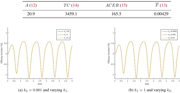
Obviously, the results depend on the objective functionalJ given in (6). Namely, they depend on the weight constants associated with the amount of infectious individualsk1 and with the cost of the controlk2. According with Figure5, results do not change qualitatively by varying constantski, i = 1, 2. Nevertheless, the magnitude of the efficacy changes slightly whenk1andk2vary independently.

Some summary measures are introduced to evaluate the cost and the effectiveness of the proposed control measure for the intervention period.

The total cases averted by the intervention during the time periodtf [24] is given by

A = tfI(0)−

∫ tf

0

time (years) 0 0.5 1 1.5 2 2.5 3 3.5 4 4.5 5 co-states 0 0.05 0.1 0.15 0.2 0.25 0.3 p 1 p2 p3 p4

(a) Variation of co-state variables.

time (years) 1 2 3 4 5 T(t) 0 0.1 0.2 0.3 0.4 0.5 0.6 0.7 0.8 0.9 1

(b) Variation of the optimal controlT(treatment).

time (years) 1 2 3 4 5 F(t) -1.2 -1 -0.8 -0.6 -0.4 -0.2 0 0.2 0.4 0.6

(c) Efficacy functionF (t)defined in (11).

Figure 4. Co-state variables, optimal controlT and efficacy functionF (t) associated to the optimal control problem (6), assuming weightsk1= 1andk2= 0.001.

whereI∗(t)is the optimal solution associated with the optimal controlT∗and I(0)is the corresponding initial condition. Note that this initial condition is obtained as the equilibrium proportionIof system (4) without treatment intervention, which is independent on time, sotfI(0) =

∫tf

0 I dtrepresents the total infectious cases over a given period oftf years.

We define effectiveness as the proportion of cases averted on the total cases possible under no intervention [24]:

F = A tfI(0) = 1− ∫tf 0 I∗(t) dt tfI(0) . (13)

The total cost associated with the intervention [24] is

T C =

∫ tf

0

CT∗(t)I∗(t) dt, (14)

whereCcorresponds to the per person unit cost of the detection and treatment of infectious individuals. Following [18,24], the average cost-effectiveness ratio is defined by

ACER = T C

A . (15)

Table4summarizes the particular case we have analyzed. These results evidence the limited effectiveness of the control variable to diminish the HRSV infectious individuals.

Table 4. Sumary of cost-effectiveness measures. Parameters according to Table1andC = 1. A(12) T C (14) ACER(15) F(13) 20.9 3459.1 165.5 0.00429 time 0 0.5 1 1.5 2 2.5 3 3.5 4 4.5 5 Efficacy function F(t) -1 -0.5 0 0.5 1 k1=10 k1=1 k 1=0.1

(a)k2= 0.001and varyingk1.

time 0 0.5 1 1.5 2 2.5 3 3.5 4 4.5 5 Efficacy function F(t) -1 -0.5 0 0.5 1 k2=0.0001 k2=0.001 k 2=0.01 (b)k1= 1and varyingk2.

Figure 5. Sensitivity analysis for the weights of the objective functional on (6). Left:k2= 0.001andk1= 0.1, 1, 10Right: k1= 1andk2= 0.01, 0.001, 0.0001.

4. Conclusion

Human Respiratory Syncytial Virus (HRSV) is the most common cause of lower respiratory tract infection in infants and children worldwide. In addition, HRSV causes serious disease in elderly and immune compromised individuals. In this work, we discussed a mathematical compartmental model for HRSV. Estimation of parameters was done for real data of Florida from September 2011 to July 2014, minimizing thel2 norm. The results show that the proposed model fits well the reality under study. Moreover, a sensitivity analysis was carried out for the basic reproduction number, in the case when the transmission parameter is taken to be the average value ofβ(t)

in the period under study, proving that the most important parameters to have into account are the rate of loss of infectiousnessνand the average of transmission parameterb0. Our results from optimal control show that treatment has a limited effect on HRSV infected individuals. This reinforces the importance of developing a licensed vaccine for HRSV, which is a subject under strong current development [17].

Acknowledgements

Rosa was supported by the Portuguese Foundation for Science and Technology (FCT) through IT (project UID/EEA/50008/2013); Torres by FCT through CIDMA (project UID/MAT/04106/2013) and TOCCATA (project PTDC/EEI-AUT/2933/2014 funded by FEDER and COMPETE 2020).

The authors are very grateful to the anonymous referees for a careful reading of the manuscript and for several questions and suggestions that improved the paper.

REFERENCES

1. L. Acedo, J.-A. Mora˜no, and J. D´ı ez Domingo. Cost analysis of a vaccination strategy for respiratory syncytial virus (RSV) in a network model. Math. Comput. Modelling, 52(7-8):1016–1022, 2010.

2. A. J. Arenas, G. Gonz´alez, and L. J´odar. Existence of periodic solutions in a model of respiratory syncytial virus RSV. J. Math.

3. A. J. Arenas, J. A. Mora˜no, and J. C. Cort´es. Non-standard numerical method for a mathematical model of RSV epidemiological transmission. Comput. Math. Appl., 56(3):670–678, 2008.

4. N. Chitnis, J. M. Hyman, and J. M. Cushing. Determining important parameters in the spread of malaria through the sensitivity analysis of a mathematical model. Bull. Math. Biol., 70(5):1272–1296, 2008.

5. R. Denysiuk, H. S. Rodrigues, M. T. T. Monteiro, L. Costa, I. Esp´ırito Santo, and D. F. M. Torres. Multiobjective approach to optimal control for a dengue transmission model. Stat. Optim. Inf. Comput., 3(3):206–220, 2015.

6. R. Denysiuk, C. J. Silva, and D. F. M. Torres. Multiobjective approach to optimal control for a tuberculosis model. Optim. Methods

Softw., 30(5):893–910, 2015.

7. FLHealthCHARTS. http://www.flhealthcharts.com/charts/default.aspx. 2015. 8. Florida Department of Health.

http://www.floridahealth.gov/diseases-and-conditions/respiratory-syncytial-virus/. Accessed: May 3, 2017.

9. W. P. Glezen, L. H. Taber, A. L. Frank, and J. A. Kasel. Risk of primary infection and reinfection with respiratory syncytial virus.

American Journal of Diseases of Children, 140(6):543–546, 1986.

10. C. B. Hall, G. A. Weinberg, M. K. Iwane, A. K. Blumkin, K. M. Edwards, M. A. Staat, P. Auinger, M. R. Griffin, K. A. Poehling, D. Erdman, et al. The burden of respiratory syncytial virus infection in young children. New England Journal of Medicine, 360(6):588–598, 2009.

11. D. Hincapi´e-Palacio, J. Ospina, and D. F. M. Torres. Approximated analytical solution to an Ebola optimal control problem. Int. J.

Comput. Methods Eng. Sci. Mech., 17(5-6):382–390, 2016.

12. A. P. Lemos-Pai˜ao, C. J. Silva, and D. F. M. Torres. An epidemic model for cholera with optimal control treatment. J. Comput. Appl.

Math., 318:168–180, 2017.

13. J. Mateus, P. Rebelo, S. Rosa, C. Silva, and D. F. M. Torres. Optimal control of non-autonomous SEIRS models with vaccination and treatment. Discrete Contin. Dyn. Syst. Ser. S, in press.

14. M. A. Mikucki. Sensitivity analysis of the basic reproduction number and other quantities for infectious disease models. PhD thesis, Colorado State University, 2012.

15. C. Modnak. A model of cholera transmission with hyperinfectivity and its optimal vaccination control. Int. J. Biomath.,

10(6):1750084, 16, 2017.

16. Y. Nakata and T. Kuniya. Global dynamics of a class of SEIRS epidemic models in a periodic environment. J. Math. Anal. Appl., 363(1):230–237, 2010.

17. K. M. Neuzil. Progress toward a respiratory syncytial virus vaccine. Clinical and Vaccine Immunology, 23(3):186–188, 2016. 18. K. O. Okosun, O. Rachid, and N. Marcus. Optimal control strategies and cost-effectiveness analysis of a malaria model. BioSystems,

111(2):83–101, 2013.

19. L. S. Pontryagin, V. G. Boltyanski˘ı, R. V. Gamkrelidze, and E. F. Mishchenko. Selected works. Vol. 4. Classics of Soviet Mathematics. Gordon & Breach Science Publishers, New York, 1986. The mathematical theory of optimal processes, Edited and with a preface by R. V. Gamkrelidze, Translated from the Russian by K. N. Trirogoff, Translation edited by L. W. Neustadt, With a preface by L. W. Neustadt and K. N. Trirogoff, Reprint of the 1962 English translation.

20. D. R. Powell, J. Fair, R. J. LeClaire, L. M. Moore, and D. Thompson. Sensitivity analysis of an infectious disease model. In

Proceedings of the International System Dynamics Conference, 2005.

21. A. Rachah and D. F. M. Torres. Dynamics and optimal control of Ebola transmission. Math. Comput. Sci., 10(3):331–342, 2016. 22. H. S. Rodrigues, M. T. T. Monteiro, and D. F. M. Torres. Sensitivity analysis in a dengue epidemiological model. In Conference

Papers in Science, volume 2013. Hindawi Publishing Corporation, 2013.

23. H. S. Rodrigues, M. T. T. Monteiro, and D. F. M. Torres. Seasonality effects on dengue: basic reproduction number, sensitivity analysis and optimal control. Math. Methods Appl. Sci., 39(16):4671–4679, 2016.

24. P. Rodrigues, C. J. Silva, and D. F. M. Torres. Cost-effectiveness analysis of optimal control measures for tuberculosis. Bull. Math.

Biol., 76(10):2627–2645, 2014.

25. C. J. Silva, H. Maurer, and D. F. M. Torres. Optimal control of a tuberculosis model with state and control delays. Math. Biosci.

Eng., 14(1):321–337, 2017.

26. C. J. Silva and D. F. M. Torres. A TB-HIV/AIDS coinfection model and optimal control treatment. Discrete Contin. Dyn. Syst., 35(9):4639–4663, 2015.

27. C. J. Silva and D. F. M. Torres. A SICA compartmental model in epidemiology with application to HIV/AIDS in Cape Verde.

Ecological Complexity, 30:70–75, 2017.

28. C. J. Silva and D. F. M. Torres. Modeling and optimal control of HIV/AIDS prevention through PrEP. Discrete Contin. Dyn. Syst.

Ser. S, 11(1):119–141, 2018.

29. P. van den Driessche. Reproduction numbers of infectious disease models. Infectious Disease Modelling, 2(3):288–303, 2017. 30. A. Weber, M. Weber, and P. Milligan. Modeling epidemics caused by respiratory syncytial virus (RSV). Math. Biosci., 172(2):95–

113, 2001.

31. T. Zhang, J. Liu, and Z. Teng. Existence of positive periodic solutions of an SEIR model with periodic coefficients. Appl. Math., 57(6):601–616, 2012.