[PENDING] Conditional Markov regime switching model applied to economic modelling.

(1)

HAL Id: hal-00747479

https://hal.archives-ouvertes.fr/hal-00747479v2

Preprint submitted on 10 Jan 2014

HAL is a multi-disciplinary open access archive for the deposit and dissemination of sci- entific research documents, whether they are pub- lished or not. The documents may come from teaching and research institutions in France or

L’archive ouverte pluridisciplinaire HAL, est destinée au dépôt et à la diffusion de documents scientifiques de niveau recherche, publiés ou non, émanant des établissements d’enseignement et de recherche français ou étrangers, des laboratoires

Conditional Markov regime switching model applied to economic modelling.

Stéphane Goutte

To cite this version:

Stéphane Goutte. Conditional Markov regime switching model applied to economic modelling.. 2012.

�hal-00747479v2�

(2)

Les Cahiers du LED

Conditional Markov regime switching model applied to economic modelling.

St´ ephane GOUTTE (Universit´ e Paris 8, LED)

Document de travail N

^◦

53 Janvier 2014

LED

Laboratoire d’´ Economie Dionysien

Universit´ e Paris 8

(3)

Conditional Markov regime switching model applied to economic modelling.

St´ephane GOUTTE

Universit´e Paris 8 (LED)

2 rue de la Libert´e, 93526 Saint-Denis Cedex, France.

December 29, 2013

Abstract

In this paper we discuss the calibration issues of regime switching models built on mean-reverting and local volatility processes combined with two Markov regime switching processes. In fact, the volatility structure of these models depends on a first exogenous Markov chain whereas the drift structure depends on a conditional Markov chain with respect to the first one. The structure is also assumed to be Markovian and both structure and regime are unobserved. Regarding this construction, we extend the classical Expectation- Maximization (EM) algorithm to be applied to our regime switching model. We apply it to economic data (Euro-Dollar/USD foreign exchange rate and Brent oil price) to show that such modelling clearly identifies both mean reverting and volatility regime switches. More- over, it allows us to make economic interpretations of this regime classification as in some financial crises or some economic policies.

Keywords:Markov regime switching; Expectation-Maximization algorithm; mean-reverting;

local volatility; economic data.

MSC classification:91G70, 60J05, 91G30.

JEL classification:F31, C58, C51, C01.

Introduction

The use of Hamilton’s Markov switching models to study economic time series data such as the business cycle, economic growth or unemployment is not new. In his seminal paper [7],

(4)

Hamilton already noticed that Markov-switching models are able to reproduce the different phases of the business cycle and capture the cyclical behaviour of U.S. GDP growth data. More recently, Bai and Wang in [3] went one step further by allowing for changes in variance and showed that their restricted model clearly identifies both short-run regime switches and long- run structure changes in U.S. macroeconomic data. Janczura and Weron in [8] showed that Markov regime switching diffusion well fits market data such as electricity spot prices and allows useful economic interpretations of regime states. Goutte and Zou in [6] compared the results given by the good fit of different regime switching models against non regime switching diffusion on foreign exchange rate data. They proved that regime switching models with both mean reverting and local volatility structures are the best choice to fit data well. Moreover, this modelling allows them to capture some significant economic behaviour well, such as crisis time periods or change in the dynamic level of variance.

Based on the above observations that Markov switching models capture economic cycles and regime switching, we would like to extend the model stated by Goutte and Zou in [6] with a conditional Markov chain structure as in Bai and Wang in [3]. Indeed, in [3], the authors ignored the points that the model could have a mean reverting effect and a regime switching local volatility structure. As mentioned before, Goutte and Zou in [6] proved that a continuous time regime switching model better fits economic time series data than a non-regime switching model. Hence, in this paper, we will define a mean reverting local volatility regime switching model where the volatility structure will depend on a first Markov chain and the drift structure will have a mean reverting effect which depends on a conditional Markov chain with respect to the first one.

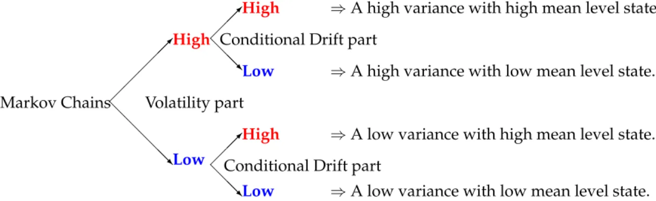
One of the objectives of this class of regime switching stochastic models is to capture various key features of the data such as mean trend gap or recession in a same economic level state of market volatility. In particular, in a possible high regime volatility state, our class of model will be able to capture different possible trends of the long mean average such as increasing or recession periods.

(5)

Markov Chains Volatility part

High

@

@@RLow

High ⇒A high variance with high mean level state.

@

@@RLow ⇒A high variance with low mean level state.

Conditional Drift part Conditional Drift part

High ⇒A low variance with high mean level state.

@

@@RLow ⇒A low variance with low mean level state.

Figure 1: Contribution of the use of a conditional Markov chain for the drift component.

Thus, unlike Goutte and Zou in [6], our more general model will allow us to distinguish different possible economic states for the drift component for the same level of volatility.

We will develop an Expectation-Maximization (EM) algorithm to apply to this class of regime switching model. Indeed, the (EM) algorithm initiated by Hamilton in [7] is a two- step algorithm: firstly an estimation procedure in which we evaluate all the probabilities of the regime switching model; secondly a likelihood maximization step to estimate all the parameters of our models. Hence, in this paper, we will follow these two steps to give the procedure in our specific regime switching model case. Finally, since one of the aims of this paper is to establish a model that could capture various key features or trends of economic time series data, such as a mean level change or growth of volatility, we will use it on some economic time series data: the Euro/Dollar foreign exchange rate and the Brent crude oil spot price in Euros.

Hence, the paper is structured as follows: in a first section, we provide some notations and introduce our model. Then, in a second part, we set out the (EM) algorithm, which is the method for estimating all the parameters of our regime switching model. Then in the last section, we apply this method to economic time series data. We also give economic interpretations and so we show the ability of this regime switching model to capture various key features such as spikes in data or changes in the volatility level or crisis time periods.

1 The model

LetT >0be a fixed maturity time and denote by(Ω,F:= (F_t)_[0,T],P)an underlying probability space. In this paper, we will follow the seminal Markov switching model introduced by Hamilton in [7]. However, in the sequel we will use a generalization of this classical regime switching model. First, we use a conditional Markov chain as initiated by Bai and Wang in [3]. Secondly, we employ a more global class of stochastic model using a mean-reverting local

(6)

volatility regime switching diffusion instead of a basic autoregressive model.

1.1 Conditional Markov chain

We begin with the construction of our Markov regime switching model. We will classify the states of the economy into exogenous and endogenous regimes characterizing long-run structure changes and short-run business cycles, respectively. The exogenous regime values will be given by a homogenous continuous time Markov chainX² on finite state K := {1,2, . . . , K}

and with transition matrixP^X² given by

P^X² =







p₁₁ p₁₂ . . . p_1K p21 p22 . . . p2K

... ... ... ... p_K1 p_K2 . . . p_KK







. (1.1)

Remark 1.1. The quantitypij represents the intensity of the jump from stateito statej.

The endogenous regime values will be given also by a homogenous continuous time Markov chainX¹on finite stateL:= {1,2, . . . , L}but its transition matrix will depend on the value of the exogenous regime. Hence, the transition matrix ofX¹ will be conditional on the value of the Markov chain X². The endogenous economic regime thus follows a conditional Markov chain, where the Markovian property applies only after conditioning on the exogenous state.

Hence, the state of the endogenous regimeX¹will be determined by conditioning on the state of the exogenous regimeX².

To define the transition matrix of X¹ we first construct a time grid partition of the time interval[0, T]. For this, we partition the time interval such that,

0 =t0< t1<· · ·< t_N =T with ∆t:=t_k+1−t_k= 1 for all k∈ {0, . . . , N}. (1.2) For alls∈ K, we can now define the probability transition to statei∈ Ltoj ∈ Lwith respect to the value of the Markov chainX² of the Markov chainX¹ as

p^s_ij =P

X_t¹_k =j|X_t²

k =s, X_t¹_k−1 =i

, ∀k∈ {1, . . . , N}, ∀s∈ K. (1.3) Hence we getK possible transition matrixP_s^X¹,s∈ Kgiven by

P_s^X¹ =







p^s₁₁ p^s₁₂ . . . p^s_1L p^s₂₁ p^s₂₂ . . . p^s_2L ... ... ... ... p^s_L1 p^s_L2 . . . p^s_LL







. (1.4)

(7)

We assume in the what follows that

Assumption 1.1. 1. For all k ∈ {1, . . . , N}, X_t²_k is an exogenous Markov process. Hence, it satisifes

P

X_t²

k+1|X_t²

k, X_t¹

k, X_t²_k−1, X_t¹_k−1, . . . , X_t²₀, X_t¹₀

=P

X_t²

k+1|X_t²

k

. (1.5)

2. For allk∈ {1, . . . , N},X_t¹_kis conditionally Markovian:

P

X_t¹

k+1|X_t²

k+1, X_t¹

kX_t²_k−1, X_t¹_k−1, . . . , X_t²₀, X_t¹₀

=P

X_t¹

k+1|X_t²

k+1, X_t¹

k

. (1.6) Point 2 of Assumption (1.1) means that the value of the Markov chainX¹ at time t_k, k ∈ {1, . . . , N}depends both on the value of the Markov chainX¹at timetk−1and of the Markov chainX² at timetk−1.

Remark 1.2. In the particular case whereK ≡ L:={1,2}and under Assumptions 1.1, this model can be defined by the joint distribution Z_t_k = X_t¹

k, X_t²

k

in the spaceS := {(1,1),(1,2),(2,1),(2,2)}. Hence, in this two-regimes case, the transition matrix of the Markov chainsX¹andX² is given by:

P^X² = p 1−q 1−p q

!

and

P₁^X¹ = p1 1−q1

1−p₁ q₁

!

, P₂^X¹ = p2 1−q2

1−p₂ q₂

! .

Moreover, we have

P Zt_k+1|Z_t_k, Ztk−1, Zt0

=P Zt_k+1|Z_t_k

=P

X_t¹_k+1|X_t²

k+1, X_t¹_k

.P

X_t²_k+1|X_t²

k

(1.7) and so the4×4transition matrix ofZ is given by

P^Z= p.P₁^X¹ (1−p).P₁^X¹ (1−q).P₂^X¹ q.P₂^X¹

!

. (1.8)

Remark 1.3. If we assume that for alli, j∈ Lands₁ 6=s₂∈ Kthatp^s_ij¹ =p^s_ij², then the Markov chain X¹ is no longer a conditional Markov chain. Indeed, its transition matrix no longer depends on the values of the Markov chainX²and so the two Markov chainsX¹ andX²are now independent. Hence, this regime switching model becomes an independent regime switching model studied, for example, by Goutte and Zou in [6], applied to foreign exchange rate data.

(8)

From an economic point of view, we can interpret the two-states case as mentioned in Re- mark 1.2 as a low/high mean and a low/high variance. Hence, whenever we know the variance level state we can determine whether we are in low or high mean level. Hence this model can capture a different level of mean in each level of variance. Indeed, with this modelling, an economic datum can be in a high variance regime but with a low mean trend and respectively in a low variance level but with a high mean level. Thus, this conditional regime switching model allows us to differentiate between these different possible states.

1.2 Regime switching diffusion

In what follows, we will work on a discretized version of the mean-reverting, heteroskedastic process given by the following stochastic differential equation

dY_t= µ X_t¹, X_t²

−β X_t¹, X_t² Y_t

dt+σ X_t²

|Y_t|^δdW_t, δ∈R⁺.

Thus, we will work on the following observed data process Y_t_k, where time(t_k)k∈{0,1,...,N} is defined by the construction (1.2), given by:

Definition 1.1. Let(Ytk)k∈{0,...,N} be our data process (i.e. a time series) and let(X_t¹_k)k∈{0,...,N} ∈ L and(X_t²_k)k∈{0,...,N} ∈ Kbe two Markov processes. Then our general model is given by

Yt_k =µ X_t¹_k, X_t²_k

+ 1−β X_t¹_k, X_t²_k

Ytk−1 +σ X_t²_k

|Y_t_k−1|^δt_k, δ ∈R⁺. (1.9) where(tk)k∈{0,...,N}follows aN(0,1).

Remark 1.4. – The regime switching model(1.9)is a continuous time regime switching diffusion with driftµ X_t¹_k, X_t²_k

+ 1−β X_t¹_k, X_t²_k

Y_t_k−1 and volatilityσ X_t²_k

|Y_t_k−1|^δ,δ∈R⁺. – The drift factor ensures mean reversion of the process towards the long run value^µ

X_tk¹ ,X²_tk β

X_tk¹ ,X_tk²

, with speed of adjustment governed by the parameterβ X_t¹_k, X_t²_k

. From an economic point of view, if the value ofβ X_t¹_k, X_t²_k

is high then the dynamic of the processY is near the mean value, even if there is a spike at timet∈[0, T]. Then, for a small time periodη, the value ofY_t+ηwill be close to the value of the mean again.

– The two Markov chains can be seen as economic impact factors. Indeed, assume that our regime switching diffusion Y models the spread of a firm A. Then, an economic interpretation of the regime switching model is that the exogenous Markov chainX² could be the credit rating of the firmAgiven by an exogenous rating company such as ”Standard and Poors”. And the endogenous regimeX¹is then an indicator of the potentially ”good health” of the firm A given the value of its credit rating (i.e. the value of the exogenous regimeX²).

(9)

The regime switching model (1.9) is thus a mean reverting model with local volatility.

Hence it is a regime switching mean reverting constant of elasticity variance model (CEV).¹ So our model is constructed to encompass most of the financial models stated in the literature.

Indeed, we can obtain:

– a regime switching Cox-Ingersoll-Ross model (CIR) by takingδ= ¹₂. – a regime switching Vasicek model by takingδ= 0.

– a regime switching mean reverting geometric Brownian motion by takingδ = 1.

Regarding Remark 1.4, givenYtk−1,Ytk has a conditional Gaussian distribution, we have:

Y_t_k ∼ N µ X_t¹

k, X_t²

k

+ 1−β X_t¹

k, X_t²

k

Y_t_k−1, σ² X_t²

k

|Y_t_k−1|^2δ .

LetY_k:={Y_t₀, Y_t₁, . . . , Y_t_k}denote the history of Y up to timet_k, k∈ {1, . . . , N}. Therefore Yn := YT represents the full history of the data process Y. Assume, now, that we work with the bivariate Markov processZ_t = (X_t¹, X_t²)defined in Remark 1.2. Hence, it takes its values in the finite spaceS :=K × L.LetΘbe the set of all parameters to be estimated. In fact, there areK(2L+ 1) + 6parameters inΘ.

Remark 1.5. IfK=L={1,2}, thenΘcontains 16 parameters to be estimated:

Θ :={µ(1,1), µ(1,2), µ(2,1), µ(2,2), β(1,1), β(1,2), β(2,1), β(2,2), σ(1), σ(2), p, q, p1, q1, p2, q2}.

Given the data process history information, the probability distribution function (pdf) of Yt_k is given by

f

Ytk|Z_t_k = (i, j);Yk−1; Θ⁽ⁿ⁾

= 1

√2πσ(j)|Y_t_k−1|^δexp (

−

Ytk−(1−β(i, j))Ytk−1−µ(i, j)2

2σ²(j)|Y_t_k−1|^2δ

)

(1.10) withX_t¹_k =i,i∈ LandX_t²_k =jforj∈ K.

2 The estimation procedure

As we said in the introduction, we will use the Expectation-Maximization (EM) algorithm initiated by Hamilton in [7]. Indeed, we will extend this algorithm to cover our regime switching model (1.9). This algorithm starts with an arbitrarily chosen vector of initial parameters

1This model was developed by Cox, J. in ”Notes on Option Pricing I: Constant Elasticity of Diffusions.” Unpub- lished draft, Stanford University, 1975.

(10)

Θ⁽⁰⁾. Then, first, in the Expectation step (E-step), the probabilities relative to the bivariate Markov chain are calculated. Hence, we evaluate the so-called smoothed and filtered probabilities.² Second, in the Maximization step (M-step), we evaluate the new maximum likelihood estimates of the parameter vectorΘbased on the probabilities evaluated in the (E-step). Finally, we repeat these two steps until the maximum of the likelihood function is reached.

2.1 The expectation step (E-step)

Assume thatΘ⁽ⁿ⁾ is the parameter vector calculated in theM-step during the previous iteration (n ∈ N). Recall that for k ∈ {0,1, . . . , N}, Y_k := {Y_t₀, Y_t₁, . . . , Y_t_k} is the information available at timet_k. Then the filtered and smoothed probabilities of our model are given by the following procedure based on the standard formulas given by Kim and Nelson (1999) in [10].

Assume that we are in the iteration n ∈ N of the estimation procedure. Then, we can evaluate:

•The Filtered Probabilities:

Based on the Bayes rule, fork= 1, . . . , N, iterate on equations:

P

Z_t_k|Y_k; Θ⁽ⁿ⁾

= f(Yt_k|Z_t_k;Yk−1; Θ⁽ⁿ⁾).P Zt_k|Y_k−1; Θ⁽ⁿ⁾ P

Z_tkf(Y_t_k|Z_t_k;Yk−1; Θ⁽ⁿ⁾).P Z_t_k|Y_k−1; Θ⁽ⁿ⁾, (2.11) whereP

Z_tk means the sum over all the possible states of the bivariate Markov chainZ and P

Z_t_k|Y_k−1; Θ⁽ⁿ⁾

= X

Z_tk−1

P

Z_t_k, Z_t_k−1|Y_k−1; Θ⁽ⁿ⁾ ,

= X

Z_tk−1

P(Z_t_k|Z_t_k−1).P

Z_t_k−1|Y_k−1; Θ⁽ⁿ⁾ ,

until P Ztn|Y_n; Θ⁽ⁿ⁾

:= P ZT|Y_T; Θ⁽ⁿ⁾

is calculated. We recall that the model definition (1.9) implies that the probability distribution functionf(Yt_k|Z_t_k;Yk−1; Θ⁽ⁿ⁾)is given by (1.10).

•The Smoothed Probabilities:

2The smoothed probability is the conditional probability that the Markov chainZt_k is in state(i, j)at timetk

with respect toYn:=YTand the filtered probability is with respect toYk,k∈ {0,1, . . . , n}

(11)

Fork=N−1, N −2, . . . ,1iterate on P

Zt_k = (i, j)|Y_n; Θ⁽ⁿ⁾

= X

Z_tk+1

P

Zt_k = (i, j), Zt_k+1|Y_n; Θ⁽ⁿ⁾

,

= X

Z_tk+1

P Z_t_k+1|Y_n; Θ⁽ⁿ⁾

.P Z_t_k+1|Z_t_k = (i, j)

.P Z_t_k = (i, j)|Y_t_k; Θ⁽ⁿ⁾ P Z_t_k+1|Y_t_k; Θ⁽ⁿ⁾ .(2.12)

2.2 The maximization step (M-step)

In the second step of the EM algorithm, new maximum likelihood (ML) estimatesΘ⁽ⁿ⁺¹⁾, for all parameters of the model, are calculated.

Remark 2.6. In a standard maximum likelihood estimation, the log-likelihood function given by

N

X

k=0

log(f(Ytk,Θ⁽ⁿ⁾))

is maximized. Here, each component of this sum has to be weighted with the corresponding smoothed probabilities. Thus, our log-likelihood function becomes

L

Θ⁽ⁿ⁾;YT

=

N

X

k=0

X

Z_tk

log

f(Yt_k|Z_t_k;Yk−1; Θ⁽ⁿ⁾)

.P

Zt_k|Y_T; Θ⁽ⁿ⁾

. (2.13) Proposition 2.1. The (ML) estimates for all the parameters of the model defined by(1.9)are given, for δ ∈R⁺,i∈ Landj ∈ K, by the following formulas:

µ(i, j)⁽ⁿ⁺¹⁾ = PN

k=1

P Zt_k = (i, j)|Y_T; Θ⁽ⁿ⁾

|Y_t_k−1|^−2δ Yt_k −(1−β(i, j)⁽ⁿ⁺¹⁾)Ytk−1

PN

k=1

P Zt_k = (i, j)|Y_T; Θ⁽ⁿ⁾

|Y_t_k−1|^−2δ , β(i, j)⁽ⁿ⁺¹⁾ =

PN k=1

P Ztk = (i, j)|Y_T; Θ⁽ⁿ⁾

|Y_t_k−1|^−2δYtk−1B1

PN

k=1

|Y_t_k−1|^−2δYtk−1B2

,

σ(j)⁽ⁿ⁺¹⁾2

= PN

k=1

P

i∈L

h

P Z_t_k = (i, j)|Y_T; Θ⁽ⁿ⁾

|Y_t_k−1|^−2δ Y_t_k−α(i, j)⁽ⁿ⁺¹⁾−(1−β(i, j)⁽ⁿ⁺¹⁾)Y_t_k−12i PN

k=1

P X_t² =j|Y_T; Θ⁽ⁿ⁾ , with

B₁ = Y_t_k−Y_t_k−1− P_N

k=1

P Z_t_k = (i, j)|Y_T; Θ⁽ⁿ⁾

|Y_t_k−1|^−2δ Y_t_k−Y_t_k−1 PN

k=1

P Z_t_k = (i, j)|Y_T; Θ⁽ⁿ⁾

|Y_t_k−1|^−2δ , B2 =

PN k=1

|Y_t_k−1|^−2δYtk−1

PN

k=1

|Y_t_k−1|^−2δ −Ytk−1.

(12)

Proof. LetZ_t_k be in state (i, j) with i ∈ Landj ∈ K then the(i, j)-th regime weighted log- likelihood function is given by

log h

L

Θ⁽ⁿ⁺¹⁾ i

= −

N

X

k=1

P

Ztk = (i, j)|Y_T; Θ⁽ⁿ⁾

log q

2π(σ(j)⁽ⁿ⁺¹⁾)²|Y_t_k−1|^2δ

+

Y_t_k −(1−β(i, j)⁽ⁿ⁺¹⁾)Y_t_k−1−µ(i, j)⁽ⁿ⁺¹⁾2

2(σ(j)⁽ⁿ⁺¹⁾)²|Y_t_k−1|^2δ

!#

.

So in order to find the (ML) estimates, the partial derivatives of the previous expression are set to zero. This leads to

∂logL

∂µ(i, j)⁽ⁿ⁺¹⁾ = −

N

X

k=1

P

Z_t_k = (i, j)|Y_T; Θ⁽ⁿ⁾−2

Y_t_k −(1−β(i, j)⁽ⁿ⁺¹⁾)Y_t_k−1−µ(i, j)⁽ⁿ⁺¹⁾ 2(σ(j)⁽ⁿ⁺¹⁾)²|Y_t_k−1|^2δ ,

=

N

X

k=1

P Z_t_k = (i, j)|Y_T; Θ⁽ⁿ⁾ Y_t_k−(1−β(i, j)⁽ⁿ⁺¹⁾)Y_t_k−1 (σ(j)⁽ⁿ⁺¹⁾)²|Y_t_k−1|^2δ

−

N

X

k=1

P Z_t_k = (i, j)|Y_T; Θ⁽ⁿ⁾

µ(i, j)⁽ⁿ⁺¹⁾ (σ(j)⁽ⁿ⁺¹⁾)²|Y_t_k−1|^2δ ,

=

N

X

k=1

P

Z_t_k = (i, j)|Y_T; Θ⁽ⁿ⁾ h

Y_t_k −(1−β(i, j)⁽ⁿ⁺¹⁾)Y_t_k−1i

(σ(j)⁽ⁿ⁺¹⁾)⁻²|Y_t_k−1|^−2δ

−

N

X

k=1

P

Zt_k = (i, j)|Y_T; Θ⁽ⁿ⁾

µ(i, j)⁽ⁿ⁺¹⁾(σ(j)⁽ⁿ⁺¹⁾)⁻²|Y_t_k−1|^−2δ.

Hence setting _∂µ(i,j)^∂^log(n+1)^L = 0, we obtain µ(i, j)⁽ⁿ⁺¹⁾=

P_N

k=1P Z_t_k = (i, j)|Y_T; Θ⁽ⁿ⁾ Y_t_k−(1−β(i, j)⁽ⁿ⁺¹⁾)Y_t_k−1

|Y_t_k−1|^−2δ PN

k=1P Z_t_k = (i, j)|Y_T; Θ⁽ⁿ⁾

|Y_t_k−1|^−2δ . Similarly straightforward calculus applied to solve _∂β(i,j)^∂^log(n+1)^L = 0allows us to obtain the expression ofβ(i, j)⁽ⁿ⁺¹⁾. Finally, estimating(σ(j)⁽ⁿ⁺¹⁾)²is quite different since it depends exclu-

(13)

sively on the exogenous Markov chainX². Thus, we get

∂logL

∂(σ(j)⁽ⁿ⁺¹⁾)² = −

N

X

k=1

X

i∈L

P

1 2(σ(j)⁽ⁿ⁺¹⁾)²

−

Yt_k−(1−β(i, j)⁽ⁿ⁺¹⁾)Ytk−1 −µ(i, j)⁽ⁿ⁺¹⁾2

2|Y_t_k−1|^2δ (2(σ(j)⁽ⁿ⁺¹⁾)²|Y_t_k−1|^2δ)²

# ,

= −

N

X

k=1

X

i∈L

P

1 2(σ(j)⁽ⁿ⁺¹⁾)²

−

Yt_k−(1−β(i, j)⁽ⁿ⁺¹⁾)Ytk−1 −µ(i, j)⁽ⁿ⁺¹⁾2

2(σ(j)⁽ⁿ⁺¹⁾)⁴|Y_t_k−1|^2δ

# ,

= −

N

X

k=1

X

i∈L

P Ztk = (i, j)|Y_T; Θ⁽ⁿ⁾ 2(σ(j)⁽ⁿ⁺¹⁾)² +

N

X

k=1

X

i∈L

P Z_t_k = (i, j)|Y_T; Θ⁽ⁿ⁾ Y_t_k−(1−β(i, j)⁽ⁿ⁺¹⁾)Y_t_k−1 −µ(i, j)⁽ⁿ⁺¹⁾2

2(σ(j)⁽ⁿ⁺¹⁾)⁴|Y_t_k−1|^2δ .

Hence again setting _∂(σ(j)^∂^log_(n+1)^L ₎₂ = 0, we obtain (σ(j)⁽ⁿ⁺¹⁾)²

N

X

k=1

X

i∈L

P

=

N

X

k=1

X

i∈L

P

×h

Yt_k −(1−β(i, j)⁽ⁿ⁺¹⁾)Ytk−1−µ(i, j)⁽ⁿ⁺¹⁾ i2

|Y_t_k−1|^−2δ,

(σ(j)⁽ⁿ⁺¹⁾)²= PN

k=1

P

i∈LP Zt_k = (i, j)|Y_T; Θ⁽ⁿ⁾

|Y_t_k−1|^−2δ

Yt_k−(1−β(i, j)⁽ⁿ⁺¹⁾)Ytk−1 −µ(i, j)⁽ⁿ⁺¹⁾2

PN k=1

P

i∈LP Zt_k = (i, j)|Y_T; Θ⁽ⁿ⁾ . Moreover, we obtain the expected result using the fact that

N

X

k=1

X

i∈L

P

:=

N

X

k=1

P

X_t²_k =j|Y_T; Θ⁽ⁿ⁾

.

Finally, in the last part of theM-step, the transition probabilities appearing in (1.1) and (1.4) need to be estimated. Following formulas in Bai and Wang (2011) [3], we get for the Markov chainX²:

p_ij = P_N

k=2P

X_t²_k−1 =i, X_t²_k =j|Y_T; Θ⁽ⁿ⁾ P

X_tk²

P_N

k=2P

X_t²_k−1 =i, X_t²

k|Y_T; Θ⁽ⁿ⁾, i, j∈ K. (2.14)

(14)

And for the Markov chainX¹: p^s_ij =

PN k=2P

X_t²_k =s, X_t¹_k =j, X_t¹_k−1 =i|Y_T; Θ⁽ⁿ⁾ PN

k=2

P

X_tk¹ P

X_t²_k =s, X_t¹_k, X_t¹_k−1 =i|Y_T; Θ⁽ⁿ⁾

, s∈ K and i, j∈ L. (2.15) Remark 2.7. In the specific case withK ≡ L:={1,2}and with the notation of Remark 1.2, we obtain

p =

PN k=2P

X_t²_k−1 = 1, X_t²_k = 1|Y_T; Θ⁽ⁿ⁾ PN

k=2P

X_t²_k−1 = 1, X_t²_k = 1|Y_T; Θ⁽ⁿ⁾

+PN k=2P

X_t²_k−1 = 1, X_t²_k = 2|Y_T; Θ⁽ⁿ⁾ ,

q =

P_N

k=2P

X_t²_k−1 = 2, X_t²_k = 2|Y_T; Θ⁽ⁿ⁾ PN

k=2P

X_t²_k−1 = 2, X_t²

k = 2|Y_T; Θ⁽ⁿ⁾ +PN

k=2P

X_t²_k−1 = 2, X_t²

k = 1|Y_T; Θ⁽ⁿ⁾, p1 =

PN k=2P

X_t²

k = 1, X_t¹

k = 1, X_t¹_k−1 = 1|Y_T; Θ⁽ⁿ⁾ PN

k=2

P

X_tk¹ P

X_t²_k = 1, X_t¹_k, X_t¹_k−1 = 1|Y_T; Θ⁽ⁿ⁾ ,

q1 = PT

t=2P

X_t²_k = 1, X_t¹_k = 2, X_t¹_k−1 = 2|Y_T; Θ⁽ⁿ⁾ PN

k=2

P

X_tk¹ P

X_t²_k = 1, X_t¹_k, X_t¹_k−1 = 2|Y_T; Θ⁽ⁿ⁾ ,

p₂ = PN

k=2P

X_t²_k = 2, X_t¹_k = 1, X_t¹_k−1 = 1|Y_T; Θ⁽ⁿ⁾ PN

k=2

P

X_tk¹ P X_t²

k = 2, X_t¹

k, X_t−1¹ = 1|Y_T; Θ⁽ⁿ⁾, q₂ =

PN k=2P

X_t²

k = 2, X_t¹

k = 2, X_t¹_k−1 = 2|Y_T; Θ⁽ⁿ⁾ PN

k=2

P

X_tk¹ P X_t²

k = 2, X_t¹

k, X_t¹_k−1 = 2|Y_T; Θ⁽ⁿ⁾.

3 Applications to economic data

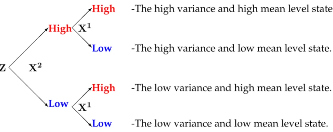
We run the estimation procedure in the specific case where each Markov chain admits two regimes, soK ≡ L={1,2}. Thus, for Remark 1.2, the bivariate Markov chainZtakes values in a four-states spaceS. In economic terms, this means there are high and low variance regimes;

and for each variance regime, there are again high and low mean regimes.

(15)

Z X²

High

@

@@RLow

High -The high variance and high mean level state.

@

@@RLow -The high variance and low mean level state.

X¹ X¹

High -The low variance and high mean level state.

@

@@RLow -The low variance and low mean level state.

Figure 2: Construction of the states of the bivariate processZ.

3.1 Euro/Dollar exchange rate

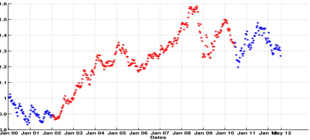
Our first data set corresponds to the Euro/Dollar foreign exchange rate for the time period between January 2000 and May 2012³.

Jan 00 Jan 01 Jan 02 Jan 03 Jan 04 Jan 05 Jan 06 Jan 07 Jan 08 Jan 09 Jan 10 Jan 11 Jan 12 May 12

0.8 0.9 1 1.1 1.2 1.3 1.4 1.5 1.6

Dates

Figure 3:Price of 1 Euro in Dollars between Jan. 2000 and May 2012.

3The data are taken from the web site http://fxtop.com/fr/

(16)

We begin by giving in Table 1 some general descriptive statistics.

Minimum Maximum Mean Std. Dev. Skewness Kurtosis Data 0.832400 1.584900 1.218614 0.196548 -0.003278 0.003184

Table 1:Summary Statistics

3.1.1 Good fit and classification measures

An ideal model is one that classifies regimes sharply and has smoothed probabilities which are either close to zero or one. In order to measure the quality of the regime classification, we propose two measures:

1. The regime classification measure (RCM) introduced by Ang and Bekaert (2002) in [1]

and generalized for multiple states by Baele (2005) in [2].

2. The Smoothed probability indicator.

These two measures are defined such that:

1. Regime classification measure: LetK(> 0)be the number of regimes, the RCM statistic is then given by

RCM(K) = 100.



1− K K−1

1 T

N

X

k=1

X

Z_tk

P

Zt_k|Y_T; Θ⁽ⁿ⁾

− 1 K

2

, (3.16) where the quantityP Z_t_k|Y_T; Θ⁽ⁿ⁾

is the smoothed probability given in (2.12) andΘ⁽ⁿ⁾ is the vector parameter estimation result. The constant serves to normalize the statistic to be between 0 and 100. Good regime classification is then associated with low RCM statistic value: a value of 0 means perfect regime classification and a value of 100 implies that no information about regimes is revealed.

2. Smoothed probability indicator: A good classification for data can be also seen when the smoothed probability is less than p or greater than 1−p with p ∈ [0,1]. Indeed, this means that the data at timek ∈ {1, . . . , N}has a probability higher than(100−2p)%in one of the regimes for the2p% error. We will call this percentage the smoothed probability indicator withp% error and we will denote it here byP^p%.

(17)

Furthermore, we calculate also the Akaike Information Criterion (AIC) and the Bayesian Information Criterion (BIC) which are given by

AIC =−2 ln(L(Θ⁽ⁿ⁾)) + 2∗k and BIC =−2∗ln(L(Θ⁽ⁿ⁾)) +kln(n), (3.17) whereL(Θ⁽ⁿ⁾)is the log-likelihood value obtained with the estimated parametersΘ⁽ⁿ⁾ found by the (EM) procedure,kis the degree of freedom of each model andnthe number of observations. We recall that the preferred model is the one with the minimum AIC or BIC value.

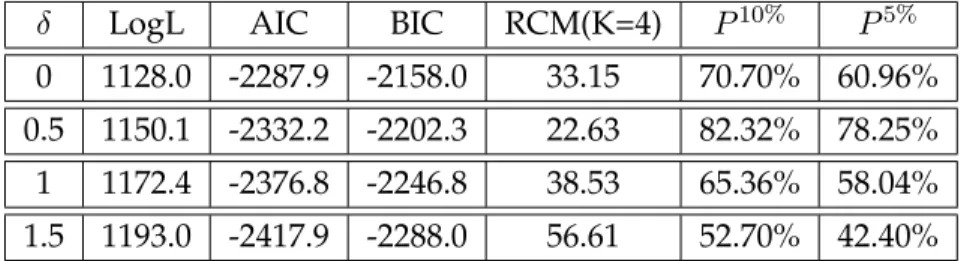
The maximum likelihood estimates determined by the (EM) algorithm are stated in Table 5 in the Appendix. We now give the log-likelihood, RCM, AIC and BIC values obtained by our estimation procedure for different regime switching models.

δ LogL AIC BIC RCM(K=4) P^10% P^5%

0 1128.0 -2287.9 -2158.0 33.15 70.70% 60.96%

0.5 1150.1 -2332.2 -2202.3 22.63 82.32% 78.25%

1 1172.4 -2376.8 -2246.8 38.53 65.36% 58.04%

1.5 1193.0 -2417.9 -2288.0 56.61 52.70% 42.40%

Table 2: Log likelihood value, AIC, BIC, RCM statistics and smoothed probability indicator given by the (EM) procedure for different values ofδ.

Let us now check which one is the best model. To make a choice, we have to take into account two things:

1. The log likelihood value given by the model. The higher this value, the better the model fits the data.

2. But, we have to weight these values with the values given by the Regime classification measure (RCM) and the Smoothed probability indicator. Effectively, they measure the good classification of the data.

Thus, even if a model has a higher log likelihood value, it is important that its RCM be close to zero to insure we have significantly different regimes. All the results are stated in Table (2). If we look at the log likelihood value alone, we can see that the highest value is obtained for the regime switching model with parameterδ = 1.5. But if we also look at the RCM values or the smoothed probability indicators, we can see that this model provides a very poor classification of the data. Indeed, we can show that the model withδ = 0.5obtains an RCM of 22.63 while

(18)

the model with δ = 1.5 obtains only an RCM of 56.61. Moreover, this model classifies only 52.70% of the data well while the model withδ= 0.5classifies 82.32% of it well.

Moreover, we can see, in Table 2, in the case where there is no local volatility contribution (i.e. model withδ = 0), that this model gives poorer results than models with a local volatility effect and particularly the regime switching model with δ = 0.5. Hence, this fully justifies adding a local volatility component to our regime switching model (1.9).

To conclude, the choice of the regime switching model withδ = 0.5 seems to be a good choice to fit this data since it obtains a log likelihood value close to the best model and it yields significantly better results in the state classification of the data than any other.

3.1.2 Economic interpretations

To interpret the results given by the (EM) algorithm, we first classify the data into two clus- ters. The first one will be called the ”smoothed low mean” cluster. It corresponds to the lowest values of the mean level of the model. In fact, for every two states of the variance Markov chain X², there are two states for the conditional drift Markov chainX¹. Thus, in this smoothed low mean cluster, we group the data where the model is in one of these two lowest values of the mean for each variance state. And we put the two highest mean level values in the smoothed high mean cluster. If we look at Graph 3, the smoothed low mean states are given by the two states: high variance low mean and low variance low mean level states.

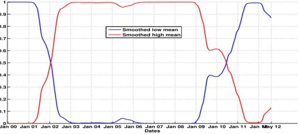
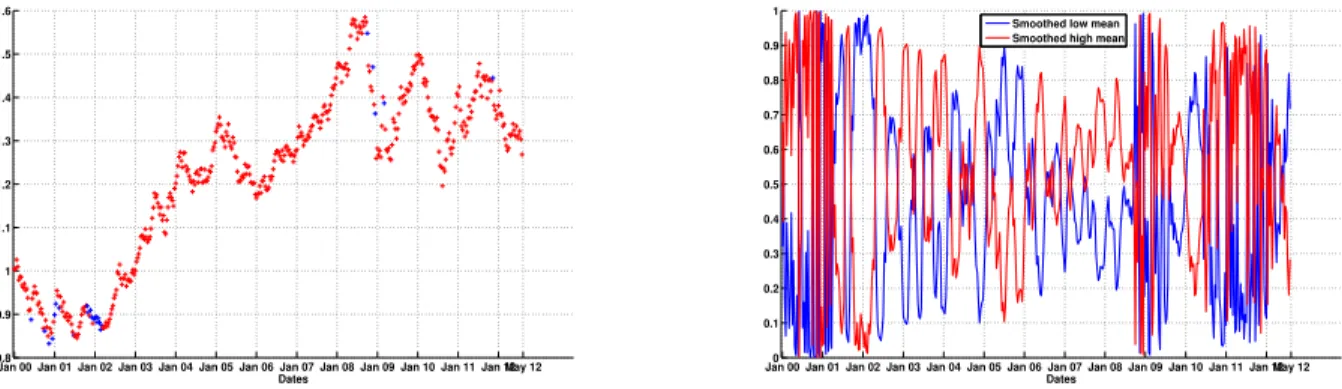
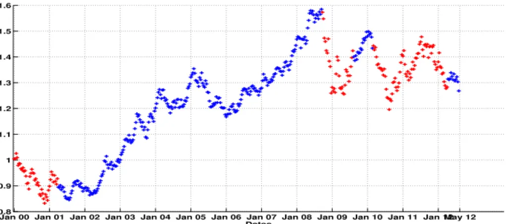
Figure 5 shows the corresponding values of each smoothed probability. Regarding our con- clusions in section 3.1.1, we interpret the results based on the regime switching model with parameterδ= 0.5. Figure 4 shows the classification result obtained for the time period consid- ered. To complete this model choice, in Figure 6 we give the corresponding result for the model withδ = 1.5. We can see that the interpretation of the regime classification seems to be, in this case, very hard or impossible since as we saw in Table 2 the regime classification measures give poor results for this model.

(19)

Jan 00 Jan 01 Jan 02 Jan 03 Jan 04 Jan 05 Jan 06 Jan 07 Jan 08 Jan 09 Jan 10 Jan 11 Jan 12May 12 0.8

0.9 1 1.1 1.2 1.3 1.4 1.5 1.6

Dates

Figure 4: Classification results given by the regime switching model withδ = 0.5. The high mean regime is in red and the low mean is in blue.

Jan 00 Jan 01 Jan 02 Jan 03 Jan 04 Jan 05 Jan 06 Jan 07 Jan 08 Jan 09 Jan 10 Jan 11 Jan 120 May 12 0.1

0.2 0.3 0.4 0.5 0.6 0.7 0.8 0.9 1

Dates Smoothed low mean Smoothed high mean

Figure 5:Smoothed probability given by the regime switching model withδ= 0.5.

(20)

Therefore, we can see in Figures 4 and 5 that in the time periods January 2000-December 2001 and May 2010-May 2012, the smoothed low mean regime prevailed. And so, in the time period January 2002-April 2010, the smoothed high mean period prevailed. This can be easily seen graphically from Figure 4. This red time period corresponds to an increasing period for the Euro/Dollar exchange rate. Effectively, the foreign exchange increases in this time period to reach a higher mean level corresponding to the high mean regime. We can also remark that the smoothed low mean regime period after May 2010 corresponds to the period after the world financial crisis before which, we were in a world economic period of upturn. Hence, the regime switching model captures this economic crisis behaviour well.

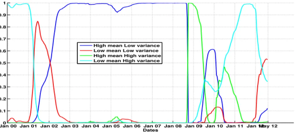
Moreover, if we look at Figures 7 and 8, we can differentiate this classification in terms of the variance level (i.e. the value of the exogenous Markov chainX²). This gives us very interesting economic and financial interpretations. We can see that during the time period just before the world economic crisis in 2010, we were in the smoothed high mean level regime but in fact from September 2008, we switched into a high variance level. Hence, just before the crisis, our regime switching model switched from a low to a high volatility level. This could imply the economic crisis started in 2010.

0.9 1 1.1 1.2 1.3 1.4 1.5 1.6

Dates

0.2 0.3 0.4 0.5 0.6 0.7 0.8 0.9 1

Dates Smoothed low mean Smoothed high mean

Figure 6: Classification results and smoothed probability given by the regime switching model with δ= 1.5.

(21)

0.9 1 1.1 1.2 1.3 1.4 1.5 1.6

Dates

Figure 7: Smoothed probability given by the regime switching model withδ= 0.5with respect to the variance levels. The high variance regime is in red and the low variance is in blue.

0.2 0.3 0.4 0.5 0.6 0.7 0.8 0.9 1

Dates High mean Low variance Low mean Low variance High mean High variance Low mean High variance

Figure 8: Smoothed probability given by the regime switching model withδ= 0.5with respect to each level of mean.

(22)

3.2 Brent oil spot price

Our second data set corresponds to the spot price in Euros of crude Brent oil between January 1990 and August 2012.⁴

90 91 92 93 94 95 96 97 98 99 00 01 02 03 04 05 06 07 08 09 10 11 12 0

10 20 30 40 50 60 70 80 90 100

Dates

Figure 9:Price in Euros of Brent oil between January 1990 and August 2012.

We begin, also, by giving in Table 3 some general descriptive statistics.

Data Minimum Maximum Mean Std. Dev. Skewness Kurtosis

Data 8.50 94.20 33.05 21.74 10937.49 688345.87

Table 3:Summary Statistics

4The data are taken from the web site http://www.indexmundi.com/

(23)

We can observe from Figure 9 spikes and changes in the level of volatility of the price which we hope to capture in our different regime states.

3.2.1 (EM) procedure results

δ LogL AIC BIC RCM(K=4) P^10% P^5%

0 -590.9 1.2 1.3 19.8 83.36% 80.79%

0.5 -361.9 691.8 813.5 25.82 77.94% 71.97%

1 -142.4 252.9 374.6 44.53 60.20% 50.73%

1.5 85.0 -202.0 -80.2 6.52 94.85% 92.28%

1.8 205.3 -442.7 -320.9 7.80 95.40% 93.11%

2 288.7 -609.3 -487.6 6.55 96.51% 94.03%

2.2 373.3 -778.5 -656.8 7.89 95.04% 90.90%

Table 4: Log likelihood value, AIC, BIC, RCM statistics and percentage given by the smoothed probability indicator obtained by the (EM) procedure for different value ofδ.

For the results stated in Table 4, the best choice of model seems to be the model with pa- rameterδ = 2. This regime switching model obtains a good likelihood value compared with the others and yields a regime classification measure close to the best one with6.55. Moreover, this model obtains the best percentage of classification with 94.03% of good classification.

3.2.2 Economic interpretations

We proceed with the same construction of classification of each regime as in the previous dataset (see section 3.1.2 and graph 3).

(24)

90 91 92 93 94 95 96 97 98 99 00 01 02 03 04 05 06 07 08 09 10 11 12 0