ISSN 1546-9239
© 2011 Science Publications
Corresponding Author: Abdul Mutalib Beksin, Department of Estate Management,Faculty of Built Environment, University of Malaya, 50603, Malaysia
A Markov Switching Regime Model of Malaysia Property Cycle
Abdul Mutalib Beksin and Bawa Chafe Abdullahi
Department of Estate Management, Faculty of Built Environment,
University Of Malaya, 50603, Malaysia
Abstract: Problem statement: Non-linear models such as the Markov Switching regime (MS) method of modeling business cycles, in principle can be used to model property cycle. Approach: The MS model can distinguish property cycle in recession and expansion phases and is sufficiently flexible to allow different relationships to apply over these phases. The Malaysian property cycle was modeled using a MS model. Results: This technique could be used to simultaneously estimate the data generating process of real GDP growth and classify each observation into one of two regimes (i.e., low-growth and high-growth regimes). Conclusions: This finding has important policy implications, since the yield spread is used to generate the time-varying probabilities of the MS model as well as the recession probabilities of the logit model. A strong relationship exists between interest rates and the business cycle, where interest rates lead the business cycle.
Key words: Property cycle, Markov Switching (MS), time-varying probabilities, policy implications, expansion phases, sufficiently flexible, MS model, recession probabilities, yield spread. Markov switching regime model, transition probabilities
INTRODUCTION
Property cycle often exhibit several common characteristics. One such characteristic is cyclical asymmetry, whereby the economy behaves differently over the expansion and recession phases of the business cycle (Kontolemis, 2001).
Although a wide variety of linear and non-linear time series techniques have been employed to model various s features of the business cycle, linear models are incapable of capturing business cycle asymmetries. Consequently, there has recently been much interest in non-linear specifications of a type that can distinguish business cycle recession and expansion phases and are sufficiently flexible to allow different relationships to apply over these phases (Simpson et al., 2001). The non-linear business cycle methods employed to capture these observed asymmetries include threshold models, smooth transition autoregressive models (Terasvirta and Anderson, 1992) and Markov Switching regime (MS) models (Hamilton, 1989).
Hamilton (1989) First introduced the MS model, which is a stochastic regime model, to business cycle modelling. He applied this model to economic growth. The model has been increasingly used to assist in the dating and forecasting of turning points in the business cycle. The model is conceptually appealing, because in that over time the variable of interest, such as some
appropriate measure of the business cycle, is regarded as having a certain probability of switching abruptly among a number of regimes. In the case of the business cycle, expansions and contractions might be considered as the two regimes, each with specific characteristics such as a unique mean and variance. In other words, the business cycle switches between a high-growth and a low-growth regime..
These discrete shifts have their own dynamics, specified as a MS process. An attractive feature of the model is that no prior information regarding the dates when the economy was in each regime, or the size of the two growth rates is required. This is in contrast with models such as probit and logit models which require and depend heavily upon the exact dates of all the regimes in the history of the series. In the case of the MS model, the probability of being in a particular regime is inferred from the data.
In this type of study, where turning points in the property cycle are modelled, it has become increasingly popular to use the yield spread as the explanatory or information variable (Estrella and Hardouvelis, 1991; Bernard and Gerlach, 1996; Estrella and Mishkin, 1998). In this study, the yield spread will be used as explanatory or information variable in the MS model. Out line: The outline of the study is as follows: The next section will summarize the theory of the lagged relationship between the yield spread and the property cycle. It also provides empirical models of the relationship between the yield spread and the property cycle.
The business cycle and the yield spread: There are two explanations for the relationship between property cycle and the term structure of interest rates (the so-called 'yield spread' between similar long-term and short-term interest rates). For the first explanation, assume that the economy is currently enjoying high growth, so that there is a general agreement among investors that the economy is heading for a slow-down or recession in the future. Investors want to hedge against recession and therefore purchase financial instruments (e.g. long-term bonds) that will deliver pay-offs during the economic slowdown. The increased demand for long-term bonds causes an increase in the price of long-term bonds, in other words, a decrease in the yield on long-term bonds. In order to finance these purchases, investors sell their shorter term assets (e.g. real estate), which results in a decline in the price of term assets and an increase in the yieldon short-term assets. In other words, if a recession is expected, long-term interest rates will fall and short-term interest rates will rise.
Consequently, prior to a recession, the slope of the term structure of interest rates will become flat (or even inverted), which means that the yield spread declines. Similarly, long-term interest rates rise while short-term interest rates fall when an expansion is expected, so that an upward-sloping yield curve predicts an expansion.
The second explanation is based on the expectations hypothesis of the term structure of interest rates. This hypothesis is based on the assumption that similar financial instruments with different maturities are perfect substitutes, so that an investor will be indifferent between investing in one long-term instrument or several similar consecutive short-term instruments, as long as their expected returns are equal (Eaton and Mishkin, 1998). This means that for similar financial instruments, the long-term yield will be the average of current and future short-term yields. Assume that a central bank tightens monetary policy by raising short-term rates. Economic agents will view this as a
temporary shock and therefore they expect future short-term rates to rise by less than the current change in short-term interest rates. On the basis of the expectations hypothesis of the term structure, long-term rates will rise by less than the current short-term rate. This will lead to a flatter or even an inverted yield curve. Since monetary policy affects economic activity with a lag of 1-2 years, the tightening of policy will cause a reduction of future economic activity and an increase in the probability of a recession. Therefore, prior to a recession (expansion), the yield spread will decline (increase).
The usefulness of the yield spread as property cycle predictor has been confirmed in empirical studies. (Estrella and Hardouvelis, 1991) were the first to empirically analyse the term structure as a predictor of real economic activity. In their study, regressions of future GNP growth on the slope of the yield curve showed that a steeper (flatter) slope implies faster (slower) future growth in real output. In addition, they also used a probit model, which showed that an increase in the spread between the long- and short-term interest rates implies a decrease in the probability of a recession four quarters later.
The markov regime switching method: Assume that there are two regimes, represented by an unobservable process denoted as St.Let St take on the values 0 and 1,
depending on the prevailing regime. In this case the DGP of the series being modeled Yt, will be different in
each regime, for example Eq. 1 and 2:
t o,o 1,0 t 1 p,0 t p t ,o t
Y = φ + φ Y −+...+ φ Y − + ε if S =0 (1)
t o,1 1,1 t 1 p,1 t p t ,1 t
Y = φ + φ Y −+...+ φ Y − + ε if S =1 (2) where s = 1 for expansionary and s = 2 for contractionary.
Also where 2
t , j N(0, )
ε ∼ σ
Following (Hamilton, 1989), assume that is a first order Markov process which means that the current regime will depend on the preceding the regime . St -1.
This model is completed by defining the transition probabilities of moving from one regime to another (referred to as 'the transition probabilities') Eq. 3 and 4:
t t 1 ij
p(S =j S− = =i) P i, j=0, 1 (3)
Thus Pij , referred to as the transition probability, is
11 t 22 t
11 21
11 t 22 t
12 22
P (w ) 1 p (w ) P P
P
1 P (w ) p (w ) P P
−
= =
−
(4)
The model 3 version, where the transition probabilities are time-invariant, is called the fixed transition probabilities model. The drawback of this model is that it implies that the expected durations of expansions and recessions can differ, but are forced to be constant over time. Intuitively, the expected duration of an expansion or contraction is generally thought to vary with the underlying strength of the economy. Filardo and Gordon (1998). The assumption that the transition probabilities are time-invariant, maybe costly from an empirical point of view. With fixed transition probabilities, the conditional expected durations do not vary over the cycle. This implies that exogenous shocks, macroeconomic policies and an economy's own internal propagation mechanisms do not affect the expectation of how long an expansion or recession will last (Filardo and Gordon, 1998).
A solution to this problem is to incorporate Time-Varying Transition Probabilities (TVTP) into the model, by using a specification for the transition probabilities that reflects information about where the economy is heading. The variations in the transition probabilities will generate variations in the expected durations (Filardo and Gordon, 1998). In contrast with the time-invariant transition probabilities in model (4) and is the information variable(s) upon which the evolution of the unobserved regime will depend. Examples of information variables are the index of leading indicators, or individual leading indicators such as the term structure of interest rates.
literature review: Property cycles have been modelled using different techniques, such as autoregressive integrated moving average model (Beveridge and Nelson, 1981; Campbell and Mankiw, 1987); cointegration techniques (King et al., 1991) and the Kalman filter, whereby real GNP is modelled as the sum of unobserved components (King et al., 1991; Harvey, 1985). These techniques share a potential shortcoming, namely the assumption that the growth rate of real GNP is a linear stationary process. Linear models are incompatible with the asymmetry between expansions and contractions that has been documented by, amongst others, (Neftc, 1984; Diebol and Rudebusch, 1990; Sichel, 1993).
Hamilton (1989) proposed a MS model that models real GNP growth as an AR(4) model, allowing for non-linearity by introducing discrete shifts in the mean between high growth and low-growth regimes. These discrete shifts have their own dynamics,
specified as a two-regime first-order Markov process. The most attractive feature of this model is that no prior information regarding the dates of the two growth periods or the size of the two growth rates is required. In addition, the low-growth rate need not be negative. In this section, a brief overview of the empirical literature on MS models for business cycles and on the relationship between the yield spread and the business cycle will be given.
Hamilton (1989) developed a MS model for dating and forecasting business cycles. He applied this model to the quarterly real GNP of the US for the period 1951-1984. In particular, he modelled GNP growth as a AR(4) two-regime MS model. In other words, GNP growth switches between two regimes, which each have a unique intercept, but the AR coefficients are constrained to be the same across regimes. The MS model calculates the probability that the economy is in a particular regime in a certain period. The econometrician then has to devise a dating rule to actually decide from which regime this observation originates. Hamilton (1989) used a very popular dating rule, which classifies a particular period as a recession (expansion) if the econometrician concludes that the economy is more likely than not to be in a recession (expansion). That is, when the probability of being in a recession (expansion) is higher than the probability of being in an expansion (recession). The dates of the turning points predicted by his MS model are usually within 3 months of the dates of the official dates set by the National Bureau for Economic Research (NBER).
Durland and McCurdy (1994) allowed the transition probabilities to be duration-dependent, so that the probability of staying in a recession, for example, declines the longer the economy is in a recession. They were able to reject the linear model in favour of a duration-dependent parameterisation of the regime transition probabilities in a regime-switching model. Layton and Katsuura (2001) compared different techniques to the MS model in dating and forecasting US business or property cycles . They estimated binomial and multinomial probit models, binomial and multinomial logit models and a two-regime MS model in which the transition probabilities are modelled as logistic functions. Their results showed that the MS model performed relatively better than the other models. The MS model overcomes a very real, practical and fundamental limitation of the logit and probit specifications as far as their use in real time property or business cycle phase shift forecasting is concerned.
Empirical investigation: In this study, the cycle will be modelled with nonlinear model using annual data for the period 1980-2007. Following the popular MS regime specification for porperty cycles, real GDP growth is modelled therefore, GDP growth γt will be
modelled and the performance of this model is evaluated later. A first-order, two-regime MS model was estimated for the Malaysian porperty cycle.The model is Eq. 5:
t 2 t 1 t 1 t 1 2 t 1
1 t 1 2 t 2 2 t 2 1 t 2 3
t 3 2 t 3 1 t 3 4 t 4 2
t 4 1 t 4 t
Y (1 S ) S [Y (1 S )
S )) (Y ( (1 S ) S ))
(Y ( (1 S ) S )) (Y (
(1 S ) S ))
− =
− − = −
− − − −
− −
= µ − + µ + φ − µ − +
µ + φ − µ − + µ + φ
− µ − + µ + φ − µ
− + µ + ε
(5)
Where 2
t
t N(0, );S 1
ε ∼ σ = if low growth regime; 0 if otherwise:
t t 1 ij, t
P(S =j S− = =i) p i, j=0,1
Following (Durland and McCurdy, 1994; Filardo, 1994), amongst others, the transition probabilities were modeled Eq. 6 and 7:
11, t t 1 1zt k 1 1zt k
P =p(S = =1) exp (α + β − ) / (α + β − )) (6)
t 2 t 1 t 1 t 1 2 t 1
1 t 1 2 t 2 2 t 2 1 t 2 3
t 3 2 t 3 1 t 3 4 t 4 2
t 4 1 t 4 t
Y (1 S ) S [Y (1 S )
S )) (Y ( (1 S ) S ))
(Y ( (1 S ) S )) (Y (
(1 S ) S ))
− =
− − = −
− − − −
− −
= µ − + µ + φ − µ − +
µ + φ − µ − + µ + φ
− µ − + µ + φ − µ
− + µ + ε
00, t t t 1 0 0zt k
0 0zt k
P p(S 0 S 0) exp( )
/(1 exp( ))
− −
−
= = = = α + β
+ α + β (7)
where the yield spread was used as the information variable Zt and the coefficients α and β were estimated
with maximum likelihood.
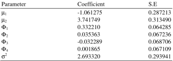
Table 1 presents significant evidence to support the assumption that two distinct growth-rate phases characterize the business cycle. The point estimates of the regime dependent means , are statistically different. The mean growth rate in the high-growth regime , is significantly positive, while the mean growth rate in the low-growth regime , is significantly positive. Because the sample dichotomises into phases that exhibit declining aggregate output and growing aggregate output, each can be labelled as low-growth and high-growth regimes of the economy.
All the estimated coefficients in the data generation process of the transition probabilities are significant. The parameters, which govern the time-variation of the transition probabilities , namely have opposite signs.
Table 1: Parameters of growth equation in Markov model Growth model
Parameter Coefficient S.E
µ1 -1.061275 0.287213
µ2 3.741749 0.313490
Φ1 0.332210 0.064285
Φ2 0.035363 0.067236
Φ3 -0.032289 0.068706
Φ4 0.001865 0.067109
σ2 2.693320 0.293941
This is consistent with the intuition that an increase in the yield spread decreases the probability of remaining in an expansion and decreases the probability of remaining in a recession. The parameters determine the unconditional mean duration of recessions and expansions.
CONCLUSION
In this study, the Malaysian property cycle has been modelled with a two-state first-order MS regime . The transition probabilities were estimated with the yield spread as explanatory variables. The results indicated that two distinct growth rate phases, these being low and high growth rate phases, characterize the property cycle. One of the most important issues for macroeconomic policy makers when making decisions about stabilization policies is to predict the most likely time of the next property cycle turning point. This finding has important policy implications, since the yield spread was used to generate the time-varying probabilities of the MS model as well as the recession probabilities of the logit model. In other words, a strong relationship exists between interest rates and the business cycle, where interest rates lead the business cycle. This implies that monetary authorities can significantly influence the course of the property cycle since they can directly influence interest rates. In addition, accurate predictions regarding the phase of the business cycle, in other words whether the economy is in a recession or not, can be made 6 months ahead based solely on the yield spread.
REFERANCES
Bernard, H. and S. Gerlach, 1996. Does the Term Structure Predict Recessions? The International Evidence. 1st Edn., Bank for International Settlements, Basle, pp: 26.
Campbell, J.Y. and N.G. Mankiw, 1987. Are output fluctuations transitory? Q. J. Econ., 102: 857-880. DOI: 10.2307/1884285
Diebol, F.X. and G.D. Rudebusch, 1990. A nonparametric investigation of duration dependence in the american business cycle. J. Polit. Econ., 98: 596-616.
Durland, J.M. and T.H. McCurdy, 1994. Duration-dependent transitions in a markov model of U.S. GNP growth. J. Bus. Econ. Stat., 12: 279-288. Eaton, J.W. and F.S. Mishkin, 1998. 1998 Readings to
Accompany the Economics of Money, Banking and Financial Markets. 5th Edn., Addison-Wesley, Reading, ISBN: 0321017544, pp: 258.
Estrella, A. and F.S. Mishkin, 1998. Predicting U.S. recessions: Financial variables as leading indicators. Rev. Econ. Stat., 80: 45-61. DOI: 10.1162/003465398557320
Estrella, A. and G.A. Hardouvelis, 1991. The term structure as a predictor of real economic activity. J. Finance, 46: 555-576.
Filardo, A.J. and S.F. Gordon, 1998. Business cycle durations. J. Eco., 85: 99-123. DOI: 10.1016/S0304-4076(97)00096-1
Filardo, A.J., 1994. Business-cycle phases and their transitional dynamics. J. Bus. Econ. Stat., 12: 299-308.
Hamilton, J.D., 1989. A new approach to the economic analysis of nonstationary time series and the business cycle. Econometrica, 57: 357-384.
Harvey, A.C., 1985. Trends and cycles in macroeconomic time series. J. Bus. Econ. Stat., 3: 216-227.
King, R.G., C.I. Plosser, J.H. Stock and M.W. Watson, 1991. Stochastic trends and economic fluctuations. Am. Econ. Rev., 81: 819-840.
Kontolemis, Z.G., 2001. Analysis of the US Business Cycle with a Vector-Markov-Switching Model. J. Forcast., 20: 47-62.
Layton, A.P. and M. Katsuura, 2001. Comparison of regime switching, probit and logit models in dating and forecasting us business cycles. Int. J. Forec., 17: 403-417. DOI: 10.1016/S0169-2070(01)00096-6
Neftc, S.N., 1984. Are economic time series asymmetric over the business cycle? J. Polit. Econ., 92: 307-328.
Sichel, D.E., 1993. Business cycle asymmetry: A deeper look. Econ. Inqu., 31: 224-224.
Simpson, P.W., D.R. Osborn and M. Sensier, 2001. Modelling Business Cycle Movements in the UK Economy. Economica, 68: 243-267.