As we said before, Frank's lemma (for diffeomorphisms) has a crucial role in proving the stability conjecture. Then the closure of the set of periodic orbits of the geodesic flow is a hyperbolic set.
Introduction
There are three main types of controllability: global controllability, local controllability at an equilibrium point, and local controllability along a reference trajectory (see [16]). For this, we recall some well-known results on global controllability and short-term local controllability at an equilibrium point.
A global controllability result : the Rashevsky-Chow Theorem
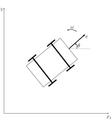
Example 2.2.4 The state of the machine is given by the position of its center of mass (x1, x2) ∈ R2 and the orientation angle θ ∈ S1 which is relative to the direction of the x1 axis position. Rotational motion: rotate the car around its center of mass with a fixed angular velocity ω = ˙θ.
Controllability of linear control systems
Let us now give two examples of controllable and non-controllable time-varying linear control systems. The time-invariant linear control system x˙ =Ax+Bu can be controlled on [T0, T1]. ii) The Kalman rank condition is met: rk.
Local controllability at an equilibrium point
Let us assume that the linearized control system in the control system x˙ = f(x, u) at (xe, ue) is controllable. Let us now define the strong jet accessibility subspace of a control system at an equilibrium point.
Local controllability around a reference control
- The End-Point Mapping
- First-order controllability results
- Some sufficient condition for local openness
- Second-order controllability results
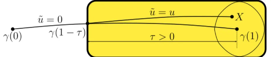
Proof of Theorem 2.5.2: From the definition of the controllability of the linearized control system along the trajectory (¯γ,u) we deduce that the map ¯ Eγ,T¯ : L2 [0, T];Rm. Summary: We provide an elementary proof of the Franks lemma for geodetic flows using basic tools of geometric control theory.
Preliminaries in geometric control theory
The End-Point mapping
First order controllability results
Proof of Theorem 1.1
Since E(ij) do not depend on time, we easily check that the matrices B0ij, Bij1, Bij2, Bij3 associated with our system are given by. In fact, since the matrices E(ij) form the basis of the vector space of symmetric matrices S(m), we easily check that the vector space.
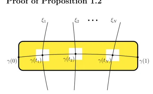
Proof of Proposition 1.2
First, a typical perturbation of the geodesic flow of a Riemannian metric in the family of smooth flows is not the geodesic flow of another Riemannian metric. But then, since a local perturbation of a Riemannian metric changes all geodesics by a neighborhood, the geodesic flow of the perturbed metric changes into tubular neighborhoods of vertical fibers in the unit tangent bundle. The collection of these levels is preserved by the operation of the differential of the geodesic flow :Dθφt(Nθ) =Nφt(θ) for each θ and t∈R.
This endomorphism can be expressed in terms of Jacobi fields of γθ which are perpendicular to γθ′(t) for each t. Its proof serves to study how small conformal perturbations of the metric g along Γ :=γ([0, T]) affect the differential of Pg(Σ0,ΣT, γ). These results are based on well-known steps towards proving the structural stability conjecture C1 for diffeomorphisms.
The proof of the above result requires that the set of periodic orbits is dense. If we reject the assumption of no conjugate points, we do not know whether the periodic orbits of expansive geodesic flows are dense (and thus whether the geodesic flow in Theorem 4.1.3 is Anosov).
Preliminaries in control theory
The End-Point mapping
In the next section, we introduce some preliminaries that describe the relationship between local controllability and some endpoint map properties and introduce the notions of first- and second-order local controllability. Our aim in the following sections is to give a top-down estimate of the size of kukL2.
First order controllability results
Second-order controllability results
Some sufficient condition for local openness
Secondly, the following non-quantitative result, evidence of which can be found, provides a sufficient condition for local openness. In the above statement, (Du2¯F)|Ker(Du¯F) refers to the quadratic map of Ker(Du¯F) to RN defined by.
Proof of Proposition 4.2.2
Consequently, the second derivative of EI,T at 0 is given by the solution (times 2) at time T of the Cauchy problem. 4.19) It is useful to work with an approximation of the quadratic form P ·D02EI,T. Indeed we will show that there is a stronger property, namely that the index of the quadratic form in (4.14) goes to infinity as δ tends to zero. The sum of the first two terms on the right-hand side of (4.20) is given by.
Finally, the sum of the first two terms on the right side of (4.20) can be written as By the same arguments as above, the sum of the third and fourth articles in Its restriction on Sp(m), ¯Π := Π|Sp(m), is a smooth mapping whose differential at X(T¯ ) is equal to the identity TX(T¯ )Sp(m), so it is an isomorphism.
In conclusion, it can be said that the control system (4.1) is controllable in the second order around ¯u≡0, which completes the proof of Theorem 2.2.
Proof of Proposition 4.2.4
Let us denote by Θ1 ⊂Θ the set of parametersθ in which EθI,T is immersion at ¯u ≡ 0, and by Θ2 its complement in Θ. For any θ ∈Θ1, since EθI,T is immersion at ¯u, we have uniform first-order controllability around ¯u for a set of parameters close to ¯θ. So we have to show that we have second-order controllability around ¯u for any parameter in a given environment of Θ2.
Furthermore, by continuity of the mapping (P, θ) 7→ P ·D20EθI,T, we can also assume that the above inequality holds for any ˜θ near θ and ˜P near P. As in the proof of Theorem 4.2.2, we must be careful because FN is valued in Sp(m).
Proof of Theorem 4.1.1
The geodesic segment γ([krg,(k+ 1)rg]) does not have its own intersection, but could intersect the segment γ([0, krg]). We conclude that the number of self-intersections of γ is bounded by N(k) +k, and in turn that it is bounded by N(k+ 1). N(k)−1} such that there is no self-intersection of γ in the closed interval. and consider local cross sections Σ0,Σ,¯ Σ,˜ ΣT ⊂ T1M tangent to Nθ, Nθ¯, Nθ˜, NθT respectively. that is, the difference between Poincar´e maps associated with geodesics of lengths T −¯t−τT and ¯t) is compact and the left and right translations in.
We denote by h·,·i,∇,Γ,H,Rm the scalar product, the gradient, the Christopher symbols, the Hessian and the curvature tensor associated with g, respectively. We will use a superscript h to denote the same objects when associated with the metric h. According to the above discussion, γ is still a geodesic with respect to h and by construction (Lemma is the support of σρ,u contained in a cylinder of radius ρ, so the above properties (1) and (2) are satisfied.
First from the compactness of M and the regularity of the geodesic flow, the compactness assumptions in Proposition 4.2.4 are satisfied. Since E(ij) do not depend on time, we easily check that the matrices Bij0, Bij1, Bij2 associated with our system are given by (remember that we use the notation [B, B′] := BB′−B′B ).
Proofs of Theorems 4.1.2 and 4.1.3
Dominated splittings and hyperbolicity
However, for geodesic flows the following statement holds: Theorem 4.4.2 Every continuous, Lagrangian, invariant, dominated splitting in a compact invariant set for the geodesic flow of a smooth, compact Riemann manifold is a hyperbolic splitting. The next step of the proof of Theorem 4.1.2 relies on the connection between sustained hyperbolicity of periodic orbits and the existence of invariant dominated splits. One of the most remarkable facts about Ma˜n´e's work on the stability conjecture (see Proposition II.1 in [46]) is to show that persistent hyperbolicity of families of linear maps is related to dominated splits. pure generic linear algebra (see Lemma II.3 in [46]).
We are now ready to combine Franks' lemma from Ma˜n´e's point of view and Theorem 4.4.3 to obtain the geodesic current version of Theorem 4.4.3. The family ψg is a collection of periodic sequences and by Franks' lemma from Ma˜n´e's point of view (Theorem 4.1.1) we have According to Theorem 4.1.1, for each δ ∈(0, δTg) (KTg . √δ)-C2 the open neighborhood of the metric (M, g) in the set of its conformally equivalent metrics covers the δ-open neighborhood Symplectic linear transformations of derivatives of Poincar´e maps between sections Σθs, Σθs+1 defined above.
Then consider δ > 0 such that the (KTg . √δ)-C2 open neighborhood of the metric (M, g) is contained in U, and we find that the family Aθ,i,g is uniformly hyperbolic. Since this holds for every periodic point θ for the geodesic flow of (M, g), the family ψg is uniform.
Proof of Theorem 4.1.3
Main ideas to show Theorem
In the case of hyperbolic symplectic matrices, the invariant subspaces of the dynamics are always Lagrangian, so we have the following elementary result of symplectic linear algebra. Then notice that any open neighborhood of the family ψ can be embedded in a neighborhood of a family of symplectic isomorphisms by the distance(ψ, η) simply by applying Lemma 4.4.9. This gives that it is enough to consider the contracting part of the dynamics of a symplectic family of periodic linear isomorphisms to extend the first part of the proof of Lemma II.3 in [46] to such families.
The second part of the proof deals with the angle between invariant subspaces of uniformly hyperbolic families (see [46] pages 532-540). The main goal of this part of the proof of Lemma II.3 in [46] is to show that an invariant splitting of a uniformly hyperbolic family is a federal dominated splitting. Due to the uniform contraction property of the stable part of the family dynamics, there exists K >0, λ∈(0,1), so that.
Moreover, the norm of such a map is the length of the largest axis of the corresponding ellipsoid. The last step of the second part of the proof is to show that the uniform hyperbolicity of families combined with the existence of a lower bound for the angle between invariant subspaces implies a dominance condition ([46] pages 534-540).
Appendix : Proof of Lemma 4.2.10
We can check with Maple that there is a ¯d∈N that is large enough so that V does not appear in the kernel of the linear form. For every integer d′ ≥ 0, let dim(d′) be the dimension of the vector space generated by V(0). By the above discussion it implies that there are four real numbers A, B, C, D which are not all zero (because a0d6= 0) such that.
But for d large enough, the intersection of 2 + 5N hyperplanes in Rd[X] with the complement of an algebraic set of dimensions of at most 6 +P + 1 is not empty.