This article is devoted to presenting some of the mathematical milestones in control theory. There it will be shown that control theory is in fact an interdisciplinary subject that has been heavily involved in the development of contemporary society.
Origins and basic ideas, concepts and ingredients
An excess of control can indeed not only entail an unacceptable cost, but also irreversible damage in the system under consideration. But of course in the development of Control Theory many other concepts were important.
The pendulum
The function w=w(t) satisfying this constraint controls the system in minimal time, i.e. the optimal control is necessarily of the form. The effect of the control in this example clearly shows the suitability of self-regulatory mechanisms.
History and contemporary applications
Maxwell in 1868, where some of the unpredictable behaviors occurring in the steam engine were described and some control mechanisms were proposed. One of the simplest applications of control theory occurs in such a seemingly simple machine as our bathroom tank.
Controllability versus optimization
Let's see the problems we had with possible system degeneracy go away (confirming the fact that this strategy leads to easier questions). Let us analyze in more detail the similarities and differences arising from the previous two formulations of the control problem.
Controllability of linear finite dimensional systems
When (1.48) is satisfied, we can confirm that, from the controllability point of view, Bt appropriately captures all the components of the adjacency stateϕ. The observability inequality guarantees that the measurements Btϕ are sufficient to detect all the components of the system.
Controllability of nonlinear finite dimensional systems
The velocity of this point must be parallel to the orientation of the rear wheels (cosϕ,sinϕ), so that. According to the previous analysis, to ensure the controllability of (1.61), it is sufficient to check that the Lie algebra of the directions in which the control can be deformed coincides with R4 at every point.
Control, complexity and numerical simulation
A more detailed description of the current state of research and perspectives in this regard can be found in the paper [1] by J. The main idea of the multi-grid method is to "separate" the low and high frequencies of the solution in the calculation process.
Two challenging applications
Molecular control via laser technology
In this case, collisions make it difficult to define their phases and, as a result, it is very difficult to choose an appropriate choice of control. For an overview of the current state of control of systems governed by the Schr¨odinger equation, we refer to the survey article [243] and the references therein.
An environmental control problem
Obviously, the main purpose of the barrier is to close the river when a dangerous rise in the water level is detected. The Thames Barrier is arguably one of the greatest achievements of Control Theory in the context of environmental protection.
The future
Biomedical research - The design of medical therapies depends very heavily on understanding the dynamics of Physiology. Control of computer-aided systems -As we mentioned above, the complexity of the control problems we face today is extremely high.
Pontryagin’s maximum principle
It is not difficult to see that this is equivalent to (1.75), given the definition of Uad. The extension of the maximum principle to control problems for partial differential equations has also been the target of intensive research.
Dynamical programming
Controllability and stabilization of finite dimensional sys-
This section is devoted to the study of some fundamental properties of controllability and stabilization of finite-dimensional systems. In Section 1 it is shown that the exact controllability property can be characterized by means of the Kalman algebraic order condition. It is shown that the system can be guaranteed to be uniformly exponentially stable if a well-chosen feedback dissipative term is added to it.
This is a specific case of the well-known equivalence property between controllability and stabilisability of finite-dimensional systems ([226]).
Controllability of finite dimensional linear systems
Note that m is the number of checks entering the system, while n is the number of components of the state to be checked. In the first case, controllability does not apply because one of the components of the system is insensitive to the control. This system is not controllable because the control does not act on the second component x2 of the state completely determined by the initial data x02.
Once again, we only have one control available for both xandy components of the system.
Observability property
Note that the checks we found have the form B∗ϕ, where ϕ is a solution of the homogeneous adjoint problem (2.9). It guarantees that the solution of the adjoint problem at t = 0 is uniquely determined by the observed quantity B∗ϕ(t) for 0 < t < T. We will use the forms (2.13) or (2.14) of the observation inequality, depending on the needs of each specific issue we will address.
The importance of the observation inequality is based on the fact that it implies the exact controllability of (2.1).
Kalman’s controllability condition
This shows that the projection of the solution xat timeT on the vector fish is independent of the value of the control u. This is a consequence of the fact that the determinant of a matrix constantly depends on its entries. This is a consequence of the fact that the determinant of an n×n matrix depends analytically on its entries and cannot vanish into a ball Rn×n.
The following inequality shows that the norm of the control is proportional to the distance between eATx0 (the state freely attained by the system in the absence of control, i.e.
Bang-bang controls
The control loop ends up going from one value to the other many times when the function B∗ϕb changes sign. It can be shown that, as expected, the controls obtained by minimizing these functionals give, in the limit whenp→1, a bang-bang control. Proposition 2.1.3 The control u2 = B∗ϕb obtained by minimizing the functional J has minimal L2(0, T) norm among all possible controls.
Stabilization of finite dimensional linear systems
It is easy to see that the solutions of this equation have an exponential decay property. Indeed, it suffices to note that the two characteristic roots have a negative real part. From this it follows that the solutions of (2.50) have the property of exponential decomposition as the explicit calculation of the spectrum shows.
If (A, B) is controllable, we have proved the uniform stability property of the system (2.32), under the hypothesis that Ais skew-adjoint.
Interior controllability of the wave equation
- Introduction
- Existence and uniqueness of solutions
- Controllability problems
- Variational approach and observability
- Approximate controllability
- Comments
Relation (2.62) can be seen as an optimality condition for the critical points of the functional J :L2(Ω)×H−1(Ω)→R,. The variational approach considered in the previous sections can also be very useful for the study of the approximate controllability property. As in the exact controllability case, the existence of a minimum of the functional Jε implies the existence of an approximate controllability.
A unique continuation principle of the solutions of (2.60), which is a weaker version of the observability inequality (2.65), will play a similar role for the approximate controllability property and it will give a sufficient condition for the existence of ' a minimizer ofJε.
Boundary controllability of the wave equation
- Introduction
- Existence and uniqueness of solutions
- Controllability problems
- Variational approach
- Approximate controllability
- Comments
The variational approach can also be used to study the approximate controllability property. Indeed, as in the exact controllable case, the existence of a minimum of the functional Jε implies the existence of an approximate controllability. The proof that the approximate controllability property implies the unique continuation principle (2.94) is similar to the equivalent in Theorem 2.2.6, and we omit it.
In the last two sections, we presented some results regarding the exact and approximate controllability of the wave equation.
Fourier techniques and the observability of the 1D wave equation 109
- Spectral analysis of the wave operator
- Observability for the interior controllability of the 1D
- Boundary controllability of the 1D wave equation
As with the proof of the previous theorem, we can reduce the problem to T =π/2 and γ≥1. On the contrary, inequality (2.99) requires that the length T of the time interval be sufficiently large. In the first inequality (2.99), T depends on the minimumγ of the distances between any two consecutive exponents (gap).
As in the context of the internal control problem, we can consider the following wave equation with a potential.
Interior controllability of the heat equation
- Introduction
- Existence and uniqueness of solutions
- Controllability problems
- Approximate controllability of the heat equation
- Variational approach to approximate controllability
- Finite-approximate control
- Bang-bang control
- Comments
As in the case of the wave equation several notions of controllability can be defined. In the case of the heat equation it is also easy to construct controls of this type. The Jbb tightening test is the same as in the functional J case.
This result shows, as expected, that the geometric control constraint is unnecessary in the context of the heat equation.
Boundary controllability of the 1D heat equation
- Introduction
- Existence and uniqueness of solutions
- Controllability and the problem of moments
- Existence of a biorthogonal sequence
- Estimate of the norm of the biorthogonal sequence: T = ∞143
We aim to change the dynamics of the system by acting on the domain boundary (0,1). The existence of a biorthogonal sequence in the family Λ is a consequence of the following theorem (see, for example, [203]). The analogies between the two problems (homogenization and numerical approximation) are clear: the grid size h in numerical approximation schemes plays the same role as the parameter ε in homogenization (see [238] and [38] . for a discussion of the connection between these problems).
In this paper, we illustrate how to do this in the context of the wave equation, a model of purely conservative dynamics in infinite dimension.
Preliminaries on finite-dimensional systems
Before we analyze (3.4) in more detail, let us see that this observability inequality does imply the controllability of the state equation. Assume the observability inequality (3.4) holds and consider the following quadratic functionalJ :RN →R:. 3.5) It is easy to see that, if ˜ϕ0 is a minimizer for J, then the check is v = B∗ϕ,˜ where ˜ϕ is the solution of the adjoint system with that datum at time=T, so is that the solution x of the equation of state satisfies the control requirement x(T) = x1. Before proving this, we note that B∗ϕ is only an M-dimensional projection of the solutionϕ that has N components.
In particular, whether a system is controllable (or its adjective observable) is independent of the time of control.
The constant coefficient wave equation
- Problem formulation
- Observability
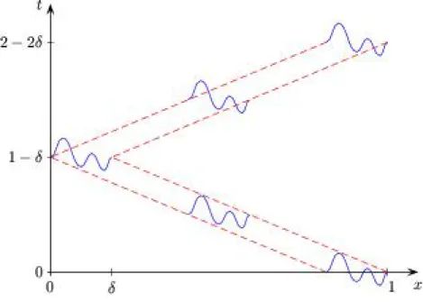
The exact controllability property of the controlled state equation (3.11) is completely equivalent 6 to the observability inequality for the adjoint system (3.8). But, in view of the time irreversibility of the wave equations under consideration, this is irrelevant. This is a consequence of the fact that the propagation velocity in this system is one and shows that the observability inequality fails for any time interval of length less than 9.
We have just seen that necessity is a consequence of the finite speed of reproduction.
The multi-dimensional wave equation
- Orientation
- Finite-difference approximations
- Non uniform observability
- Fourier Filtering
- Conclusion and controllability results
- Numerical experiments
- Robustness of the optimal and approximate control prob-
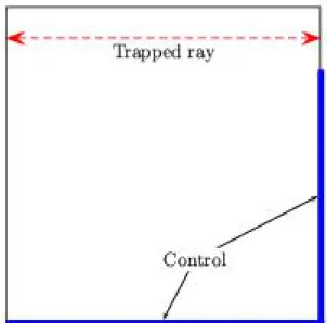
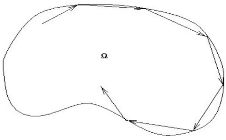
The projections of the bi-characteristic rays in the (x, t) variables are the rays of the geometric optics that play a fundamental role in the analysis of the observation and control properties through the geometric control condition (GCC). The total energy of this solution is of order 1 (because each component is normalized in the energy norm and the eigenvectors are orthogonal to each other). If the checks are bounded, they converge in L2(0, T) to the checkv of the continuous wave equation.
The approximate control of the semi-discrete system can be achieved by minimizing the functional.
Space discretizations of the 2D wave equations
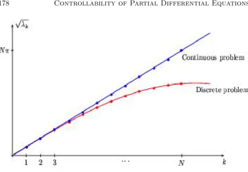
It is well known that this semi-discrete scheme provides a convergent numerical scheme for approximating the wave equation. Note that the discrete version of the energy observed at the boundary is given by . The eigenvalue problem associated with (3.82) is. 3.100) Again, the discrete eigenvalues and eigenvectors converge at h → 0 to those of the continuous Laplacian.
However, when 0 < γ <8, solutions in the class Cγ(h) do not contain the contribution of the high frequenciesλ >.
Other remedies for high frequency pathologies
- Tychonoff regularization
- A two-grid algorithm
- Mixed finite elements
Other models
- Finite difference space semi-discretizations of the heat
- The beam equation
Further comments and open problems
- Further comments
- Open problems
Approximate controllability of the linear heat equation
- The constant coefficient heat equation
- The heat equation with rapidly oscillating coefficients . 236
- The constant coefficient heat equation
- The heat equation with rapidly oscillating coefficients in
- Uniform controllability of the low frequencies . 250
- Control strategy and passage to the limit
Rapidly oscillating controllers
- Pointwise control of the heat equation
- A convergence result
- Oscillating pointwise control of the heat equation
Finite-difference space semi-discretizations of the heat equation 270
Introduction and main result
Observability of the adjoint system
Null-controllability
Further comments
Boundary control and observation through the wave component 287
Ingham-type inequality for mixed parabolic-hyperbolic spectra 289