Décollement de matériaux viscoélastiques : du liquide visqueux au solide élastique mou

Thèse de doctorat de l'Université Pierre et Marie Curie et de l'Université de la Sarre. Pour le mécanisme d'interface, nous réussissons à expliquer la dépendance de l'énergie d'adhésion à la vitesse à travers les propriétés volumiques du matériau.

General introduction

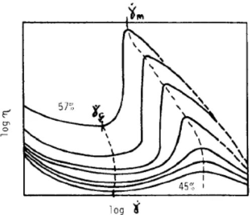
A change in the wavelength of the resulting surface instability revealed the transition between liquid and solid behavior. We describe the change in the shape of the curve as the viscoelastic properties of the material vary and clearly identify three different debonding mechanisms.

Figure 1.1.: Surface instabilities in viscoelastic liquids.

Viscosity, elasticity, and viscoelasticity

Liquids
Elasticity
Viscoelasticity
Characterization by rheometry

In the linear regime, stress is related to strain through the tensile modulus. It represents the proportionality constant between the total stress and the total strain in the system.

Figure 2.2.: Shear thinning and shear thickening liquids.

Theoretical concepts of adhesion

Measuring adhesive properties

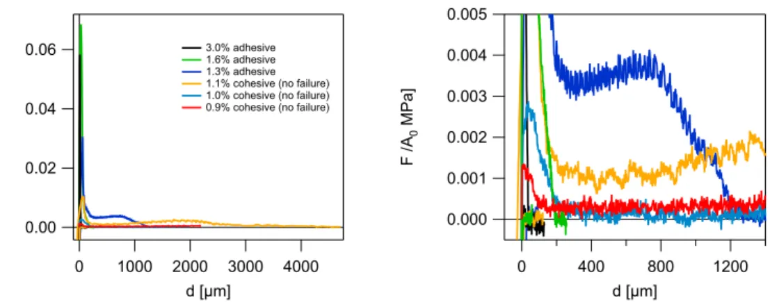
The resistance to shear obtained in this way is commonly used as a measure of the material's ability to resist flow. The force and the displacement of the probe are recorded during the entire test, so it is possible to trace characteristic curves for the entire unbinding process and calculate the energy per unit area needed to release the probe from the adhesive.

Figure 3.1.: Different techniques to characterize the performance of pressure sensitive adhe- adhe-sives, see reference [41].

Debonding mechanisms

From rheological properties to debonding mechanisms

In contrast, if G > G0, it similarly follows that dA < 0 and the crack progresses to the center of the contact area. Gc− G0 is then the driving force of the crack, whereas G0Φ(aTV) stabilizes the crack speed at V and thus acts as a brake in the system.

Viscous and elastic instabilities in confined geometriesconfined geometries

Linear stability analysis

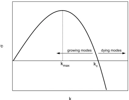
If σk is negative, the amplitude of the corresponding perturbing mode k is damped away and the ground state is stable against this perturbation. For many systems there exists a critical control parameter below which the system is stable against all perturbing conditions and above which a destabilizing condition exists.

The Saffman–Taylor instability

The velocity of the fluid and the contact line is proportional to the pressure gradient∇p. First, the perturbation in the pressure field must have the same periodicity in the spatial y -direction as the initial perturbation of the contact line.

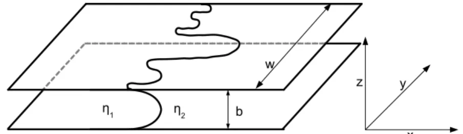
Figure 4.1.: Schematical view of a Hele–Shaw cell filled with two liquids of different viscosi- viscosi-ties

Elastic interfacial instability

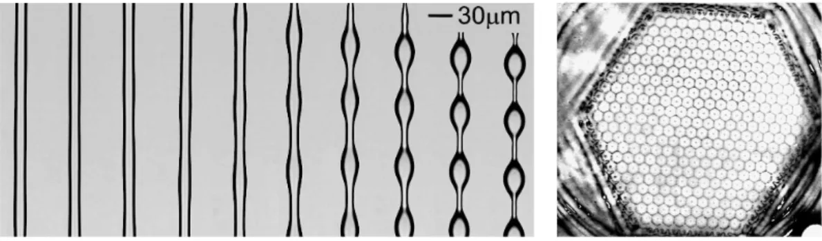
A rigid flat contactor is placed at a distance from the free surface of the film and the free surface of the film is allowed to deform. They find that for small enough distances d, the homogeneous solution is unstable and ripples of the contact line appear. A transition from viscous to elastic behavior is reflected in a change in the wavelength of this surface instability.

The strains decay exponentially into the bulk of the elastomer, also with the typical length scale lp.

Figure 4.7.: Contact instabilities in confined elastic systems.

Materials

Preparation of the PDMS samples
Characterizing the samples
Liquid-solid transition varying the number of crosslink points
Varying the rheological properties

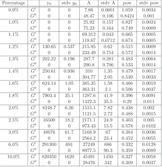
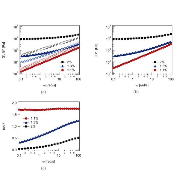
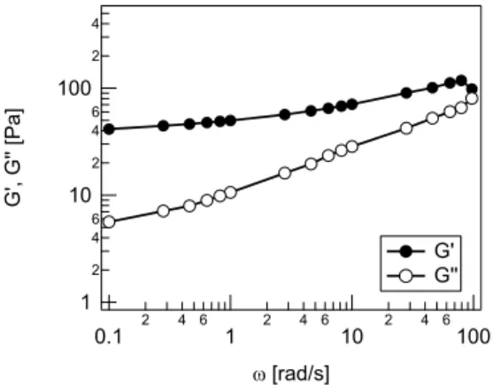
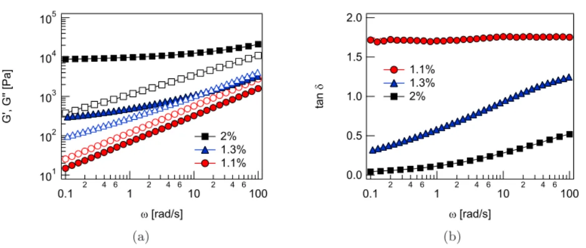
In this way we had access to the material properties as a function of the frequency. The elastic modulus remains almost independent of the frequency above a hardener content of about 2%. The elastic modulus as a function of the amount of crosslinker from different sources. b) tanδ as a function of the amount of crosslinker.

The complex modulus decreases with increasing temperature for both investigated materials, albeit weakly.

Figure 5.2.: The sample shape as measured in a profilometer for different percentages and different applicator gaps

Experimental setup and image treatmenttreatment

The probe tack test

An optical fiber measures the relative displacement of probe and table, and a load cell the force on the probe. The table with the fixed sample can be tilted with three screws to adjust the probe surface and the adhesive layer. In the current setup, the optical fiber is attached to the sample holder and the reflecting silicon wave is attached directly to the probe.

In Chapter 7 we study the pattern formation that occurs at the edge of the probe.

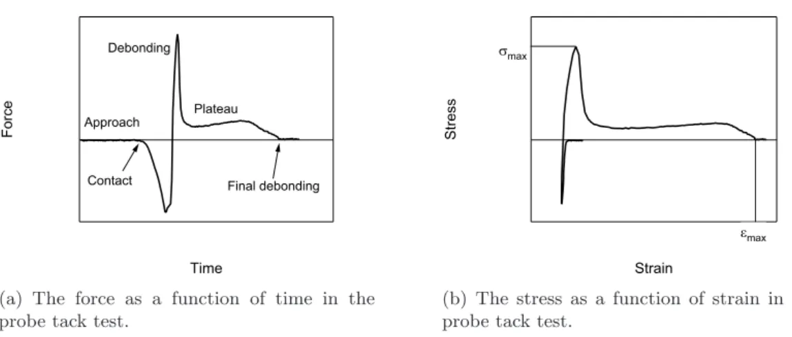
Figure 6.1.: Typical force-time and stress-strain curves in the probe tack test.

Image treatment

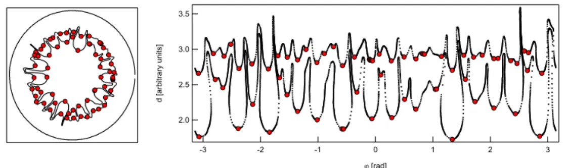
The number of fingers is then determined using the so-called FindPeak built-in algorithm. In most cases, the distance to the center of the image is not a function of the angle ϕ from 0◦ to 360◦ as the fingers soon bulge out, see Figure 6.5. Thus, we determine the minima of the distance to the center as a function of i, the internal ordinal number of each point in the dataset provided by Igor.

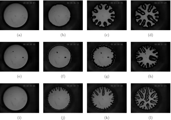
From such an image treatment we get information about the contact area, the perimeter length and the number of fingers for a large number of experiments.

Figure 6.5.: The contour lines and the position of the minima in x-y and ϕ-d representation at two different times.

Pattern formation

Introduction
Experimental
Two regimes of debonding
Transition
Nonlinear patterns
Conclusion and discussion

Hence the following subtle problem arises: the v-dependence of the wavelength is exclusively included in the v-dependence of G?. We measured the wavelength of the plasma experiment and compared it with the ST prediction. So far, we investigated the destabilization process at the onset of the instability.

The interest of the circular system lies in the fact that it is intensively used for the study of commercial adhesives.

Figure 7.1.: Formation of air fingers in the bulk deformation case, r = 0.11. Upper row:

The complete debonding process – force curves and adhesion energiesforce curves and adhesion energies

Introduction
Experimental protocol
Force-displacement curves
Quantitative analysis of the stress-strain curves
Conclusion

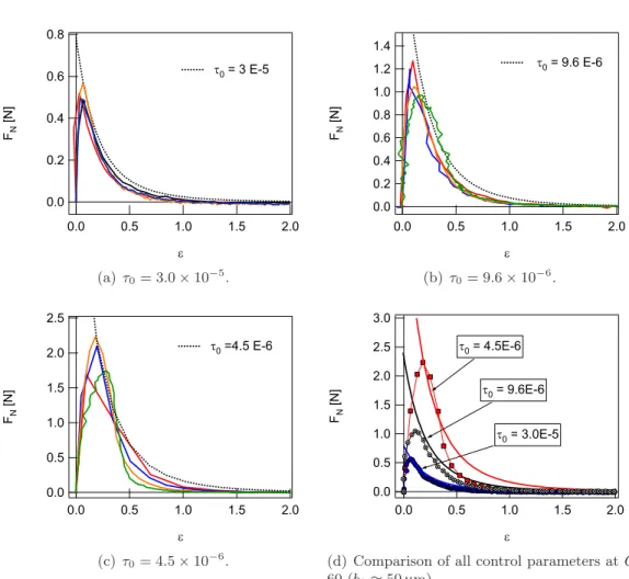
In this section, we investigate the change in the shape of the force curves with varying material properties. In the following, we describe the characteristics of the various stress-strain curves for the entire debonding process. At the end of the unbinding process, a stretched fibril may detach from the probe or break in half.

The speed dependence of What is included in the value of the maximum elongation ²max.

Figure 8.2.: Comparison of the stress-displacement curves for different materials between 0.9% and 3.0% of curing agent

A novel technique for direct visualization of the contact line

Introduction – the need for 3D-visualization
Setup
First results
Conclusion

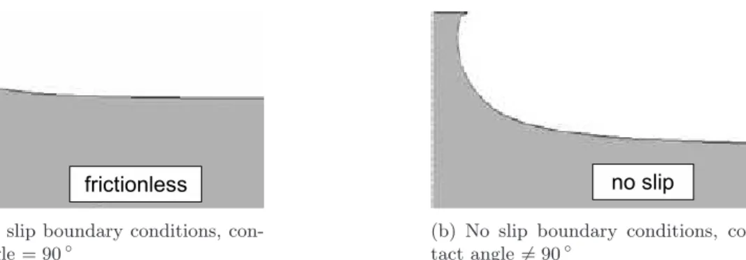
The shape of the contact line during debonding in the probe pin geometry was considered from a theoretical point of view for solids. In particular, they studied the shape of the air-elastomer contact line as the interfacial crack propagates. All these studies testify to the importance of a clearer understanding of the exact shape of the contact line and the contact angle.

We investigated the shape of the contact wire for materials with different amounts of hardener.

Figure 9.2.: Large strain simulations of the debonding of a soft elastomer for free slip and no slip boundary condition

The time evolution of the fingering pattern in a Newtonian oil

Introduction

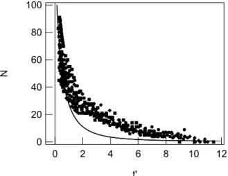
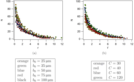
The reason for this is that the radius R of the attractor circle changes with time and the wavelength must be calculated relative to the circumference. They both introduced a dimensionless surface tension τ0 that controls the number of fingers at the onset of instability. The initial number of fingers N0 = 2πR0/λ, where λ is the fastest growing wavelength at the onset of instability, is related to τ0 as.

They also took into account the three-dimensional shape of the meniscus between oil and air.

Materials and methods

Initially, the system is at rest and the 2D projection of the oil-air interface is ideally a perfect circle. The contact line is not visible because it lies on the edge of the probe. A crucial point was determining the starting time t0 = 0, which is the moment when the motors start to lift the top glass plate and the oil starts moving.

First move and Toast still indicate the timestamps of the two images between which the oil began to move first.

Table 10.1.: Fit parameters to an exponential law describing the temperature dependence of the viscosity for two Newtonian oil, see figure 10.2.

The number of fingers in comparison to linear 2D theory

Initially, the average number of fingers in experiments and theory is of the same order of magnitude. A closer look at the images from the experiments shows that the decrease in the number of fingers is caused by the death of the fingers. Even if they don't grow, they add to the total number of fingers.

We have shown that the number of growing fingers is described by a time-dependent control parameter derived from linear stability analysis.

Figure 10.5.: N versus t 0 for τ 0 = 9.6 × 10 −6 . The solid line corresponds to the theoretical prediction from linear stability analysis equation 10.9.

Confinement dependence

The dependence of the total number of fingers is more or less pronounced depending on the control parameter. This is also seen in the time-lapse images in Figure 10.10 as in the number of fingers as a function of time in Figure 10.11. In contrast, the effect of confinement is more difficult to discern at the highest control parameter of 3.0×10−5.

The finger amplitude is smaller for higher control parameters and counting becomes more difficult, see figure 10.10.

Figure 10.9.: N versus t 0 . Circles correspond to R 0 = 3 mm, squares to R 0 = 5 mm, and diamonds to R 0 = 1.5 mm

Finger growth

To the left of the minimum, the growth rate decreases as the control parameter increases. First, the position of the fingertips is similar for different conditions (blue and red). However, the origin of the different initial conditions remains unclear in the experiment so far.

In the previous section, we discussed the possible effect of initial disturbance on finger growth.

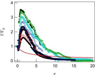
Figure 10.13.: The dimensionless perimeter as a function of dimensionless time for different realizations of τ 0 = 9.6 × 10 −6

Lifting force

In Figure 10.19(a), the experimental results are well below the calculated force, but the overall shape is well predicted. For even larger numbers of fingers [Figure 10.19(c)], the gap between experimentally measured and calculated force becomes more important. The parallel evolution of decreasing force and increasing finger amplitude thus indicates that the fingering process is indeed responsible for the decrease in force, as predicted from simulations by Linderet al.

Note that the radius R0 in Figure 10.20 is different from our experiments, so the absolute values of the force cannot be compared.

Figure 10.19.: The normal force on the probe versus the strain during the debonding process.

A viscoelastic shear thinning liquid

Finger pattern in Newtonian oil. b) 1% Carbopol solution Figure 10.21.: Comparison of |η?|versusω and η versus ˙γ for Carbopol solutions. With Newton's oil, we determined the total number of fingers and the number of growing fingers. As for Newtonian oil, the total number of fingers is greater than predicted from linear theory due to stagnant fingers, as explained earlier.

At this point in the study, we cannot assess whether the constraint has the same important rule as Newton's olives.

Figure 10.22.: G 0 and G 00 versus ω for the 1% Carbopol solution.

Conclusion

A second effect that we have studied in this chapter is the influence of finger instability on lifting force. Therefore, we investigate here whether their theory can predict the influence of our observed confinement. Previously we showed that the number of fingers changes significantly, especially at the beginning of the experiment.

The linear relationship between the number of fingers and time shows that these fluctuations can be attributed to the time dependence of the number of fingers.

Figure 10.27 compares the experimental results to linear 2D theory and numerical 3D predictions

Conclusion

On calcule la longueur d'onde de la déstabilisation initiale λ = 2πR/n, R est le rayon du poinçon. Au moment de la séparation, nous obtenons des images 3D de la ligne de contact qui avance. Pour compléter l'étude de la formation des structures, nous avons étudié une huile newtonienne dans une telle cellule.

Les résultats que nous avons obtenus sont très utiles pour l’amélioration des adhésifs, des matériaux très complexes, ainsi que pour la compréhension fondamentale de la formation de structures dans les matériaux viscoélastiques.