Cette propriété est à l’opposé du comportement typique de l’équation de Burgers invisible donnée par Dans ce paragraphe, nous décrivons rapidement l'établissement de l'équation de Burgers pour modéliser le trafic routier.
Systèmes de contrôle autour de l’équation de Burgers visqueuse
Le système (1.19) est globalement contrôlable par zéro en peu de temps si et seulement si le système (1.20) est globalement contrôlable par zéro en peu de temps. De plus, pour le système (1.20), la contrôlabilité avec la commande v1 à droite est équivalente à la commande v0 à gauche.
Quelques résultats de contrôlabilité à zéro connus
En ajoutant ce contrôle interne aux deux contrôles aux frontières, cela démontre qu'un contrôle global de toutes les trajectoires peut être obtenu en peu de temps. Avec la croissance comparative de (1,42), nous pouvons nous rapprocher le plus possible de zéro.
Nouveau résultat : contrôlabilité globale mixte avec deux contrôles
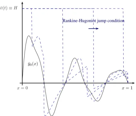
La première étape de la preuve consiste à étudier le système hyperbolique limite (qui s'obtient formellement en prenant la limite ε = 0), sur l'intervalle fixe [0, T]. Une fois que nous avons atteint un état uniforme dans l’espace, nous utilisons le contrôle u(t) pour descendre.
Nouveau résultat : non contrôlabilité avec un seul contrôle interne
Puisque a dépend linéairement de u et b dépend carrément de a, il est raisonnable de croire qu'à l'instant finalt= 1 on peut écrire une formule du type. Une piste serait de procéder en deux phases : une première phase où l'on utilise un contrôle de très grande amplitude et fortement oscillatoire pour créer des couches limites bien concentrées aux bords du domaine, puis une deuxième phase où l'on laisse les couches limites se dissiper naturellement. .
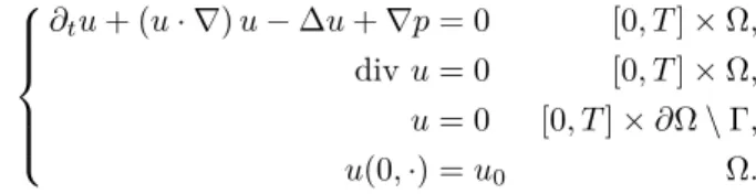
Contrôlabilité de l’équation de Navier-Stokes
Éléments historiques et premiers résultats
La condition Navier-Stokes la plus courante est la condition de glissement ou de Dirichlet indiquée par. Le choix de la condition aux limites utilisée est alors déterminant pour l’étude du comportement des couches limites.
Résultats de contrôlabilité connus
Dans le même esprit, Fursikov et Imanuvilov [86] prouvent le résultat nul de la contrôlabilité globale dans le temps court où le contrôle agit sur l'ensemble du mur (Γ = ∂Ω). Pour les conditions de Dirichlet (mathématiquement les plus difficiles), Guerrero, Imanuvilov et Puel ont prouvé dans [100] (ou [101]) pour un carré (ou cube) dont le côté (ou face) n'est pas incontrôlé, un résultat qui ressemble à un résultat global contrôlabilité, approchée en peu de temps.
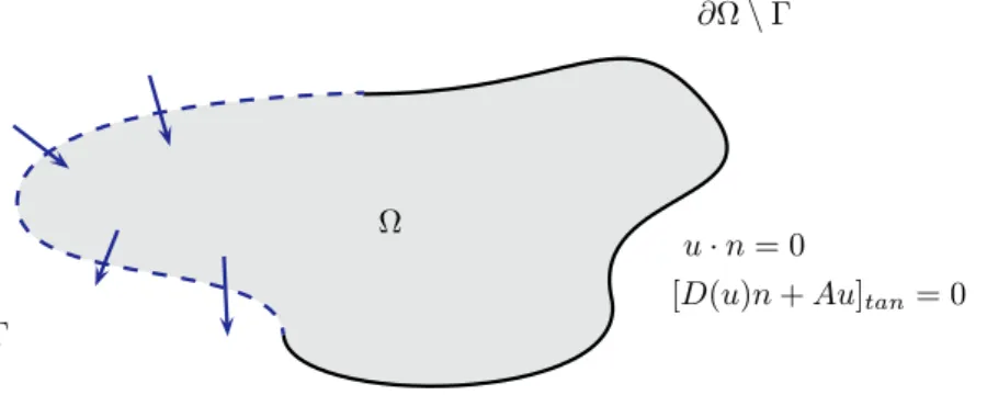
Nouveau résultat : contrôlabilité globale à zéro avec Navier au bord
En fait, il est précédé d'un facteur ε5/4 et est donc petit (à condition de montrer que son équation d'évolution est bien posée). Correction de couche limite A l'ordre O(√ . ε) nous introduisons le profil de correction de couche limite.
Perspectives méthodologiques
Méthode “du noyau asymptotique”
Cependant, puisque nous utilisons ici une vérification et que nous construisons explicitement une grande partie de la solution, nous pouvons espérer démontrer qu’il s’agit d’une solution robuste. On pourrait espérer démontrer que le résultat est vrai si seulement Γ est supposé être un ensemble ouvert non vide du mur.
Méthode “de la dissipation préparée”
Décomposer l'état sous la forme ηa+η2b ; où a est contrôlable et b libre d'ordre linéaire, et η est un petit paramètre représentant l'ampleur du contrôle. Vérifier que le noyau Kε se comporte comme K0 pour ε suffisamment petit en estimant la taille des noyaux restants, par exemple en utilisant des méthodes telles que les opérateurs intégraux faiblement singuliers.
Contrôle de l’équation de Burgers en présence d’une couche limite
- Introduction
- Description of the system and our main result
- An open-problem for Navier-Stokes as a motivation
- Previous works concerning Burgers’ controllability
- Strategy for steering the system towards the null state
- A comparison lemma for controlled Burgers’ systems
- Analysis of the hyperbolic limit system
- Small time versus small viscosity scaling
- Obtaining the entropy limit
- Small time null controllability
- Hyperbolic stage and settling of the boundary layer
- Steady states of system (2.5)
- First step : overriding the initial data
- Second step : going back to the null state
- Passive stage and dissipation of the boundary layer
- Cole-Hopf transform
- Fourier series decomposition
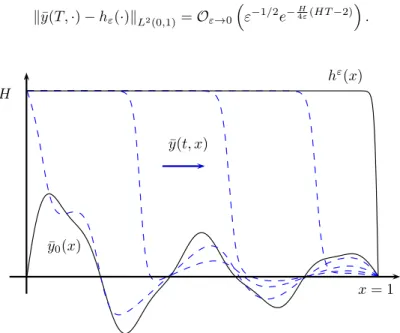
- Approximate controllability towards the null state
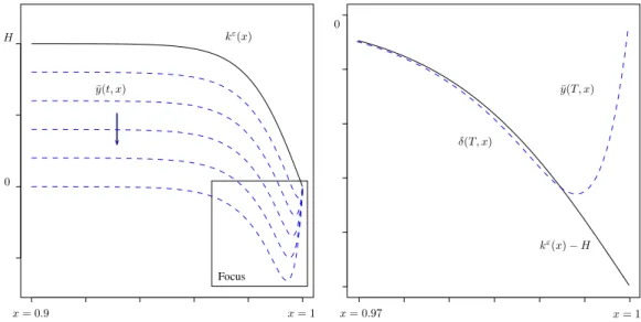
- Parabolic stage and exact local controllability
- Fursikov and Imanuvilov’s theorem
- Using Cole-Hopf and a moments method
- Conclusion and perspectives
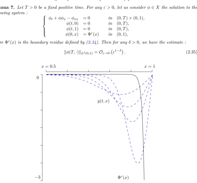
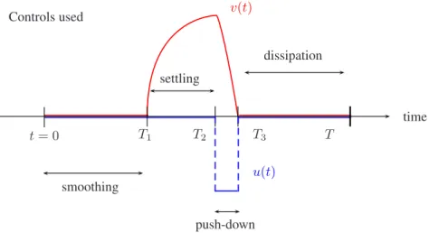
Regularization properties of the viscous Burgers equation dissipate the boundary layer and the magnitude of y(t,·) decreases. Such a study of the linearized problem around a steady state for the Burgers equation can be found in [114]. The second part [T1, T2] of length ε is the part where the subsidence of the boundary layer takes place.
A fourth part [T3, T] of length at least T /3 (when ε is small enough) is the passive rate for boundary layer dissipation. Another idea is the dissipation of the boundary layer by the fluid system itself during the passive stage.
Contrôle de l’équation de Burgers avec un unique contrôle scalaire
Introduction
- Description of the system and our main result
- Motivation : small time obstructions despite infinite propagation speed
- Previous works concerning Burgers’ controllability
- A quadratic approximation for the non-linear system
- A finite dimensional counterpart
- Strategy for the proof
Fernández-Cara and Guerrero derived the asymptotics of the minimum zero controllability time T(r) for initial states of norm H1 lower than r (see [77]). In [140], Perrollaz studies the controllability of the inviscid Burgers equation in the context of entropy solutions with an additional control u(·) and two boundary controls. So, if η describes the size of the control as in Definition 3, let's call our control ηu(t), minus the size of u.
The controllability of systems like (3.11) is deeply connected to the repeated Lie brackets of the vector field def0enf1 (see [55, Section 3.2] for an overview). Moreover, the amount by which b increases is linked to the order of the first bad lie bracket and can be expressed as a weak norm depending on the control.
Preliminary technical lemmas
- Properties of the functional space
- Smooth setting for the heat equation
- Weaker settings for the heat equation
- Burgers and forced Burgers systems
In Section 3.3, we show that formula (3.16) holds, and give an explicit construction of the Kε kernel. In Appendix 3.8, we give a brief presentation of the theory of weakly singular integral operators and a sketch of the proof of the main evaluation lemma that we use. Although (3.28) is not a direct consequence of the combination of (3.20) and (3.23) (which would give a weaker conclusion), it can be obtained by standard application of the maximum principle that can be applied in this strong setting.
For the sake of completeness, we give a short proof of the existence of a solution to system (3.1) and a precise evaluation of forced Burgers-like systems, which will be needed in the following. The second score (3.45) is due to the principle of the maximum that can be used in this powerful setting.
From Burgers to a kernel integral operator
- A general method for evaluating a projection
- Choice of a projection profile
- Rough computation of the asymptotic kernel
Using this system, we can convert the temporal projection of the statenz modρ into a projection of the source termf onto the full square. The integrations by parts performed above are valid because of the zero bound and initial conditions chosen in systems (3.47) and (3.50). Thus we have proved Lemma17 and we have a very precise description of the kernel involved.
This kernel also depends strongly on the viscosityε, which is involved in the calculation of both Φ and of the elementary solution G. However, since both ρ and ρxx satisfy zero boundary conditions, the calculations of the different kernel residuals appear to be easier.
Coercivity of the asymptotic kernel
- The limite kernel is positive definite
- Some insight and facts
- Highlighting the singular part of the kernel
- Riesz potential and fractional laplacian
- Positivity of the smooth part
- Conclusion of the proof
Although it is true that the kernels involved in the proof of Lemma 21 are strictly negative (or positive), we cannot adapt the proof to prove that N is definite. Combining the idea that the eigenvectors of N should behave asymptotically like oscillating sines and formula (3.72), we expect it to be possible to prove Lemma 20 by such an asymptotic study. To prove its tightness, we will have to isolate the most special part of it.
To complete the proof of Lemma 20, we show that the smooth part of our kernel is of positive type. We can also rely on smoothness arguments to prove that its behavior does not modify the asymptotic behavior of the eigenvectors and eigenvalues of the singular part.
Exact computation of the kernel and estimation of residues
- Smoothness of weakly singular integral operators
- Asymptotic expansion of the kernel
- Handling the first kernel
- Handling the second kernel
- Handling the third kernel
- Handling the fourth kernel
- Handling the fifth kernel
- Handling the sixth kernel
- Conclusion of the expansion of the asymptotic kernel
Thanks to the change of variables already mentioned, the same property holds for K0 with the symmetric conditionF(0) = 0. This lemma is due to the exponentially decaying factor within the source termσ defined by (3.96), which allows as many differentiations with regard to toxortas had to be made. The first integral gives rise to the main coercive part of the kernel and has already been calculated exactly in Section 3.3.
However, the calculations associated with R2 are very similar to those we perform for R3. Continuing as above, differentiating equation (3.135) with respect to tos2 (or similarly β), then combining Lemma29 and Lemma28 yields.
Back to the full Burgers non-linear system
- Preliminary estimates on the first orders
- Non-linear residue
- A first drifting result concerning reachability from zero
- Persistance of projections in absence of control
- Proof of Theorem 6
Let's expand yasa+b+r, where stands for the linear approximation of the first order, b stands for the second quadratic order and is the (small) remainder. In a sense, the state moves towards the +ρ direction, as a result of the operation of the control. We begin by noting that the projection of the state against any fixed profile µ∈L2(0,1) remains almost constant in the short time when no control is applied.
We consider the initial data of the form δ=δρ, where δ >0 can be chosen as small as we need, and ρ is defined in (3.59). Therefore, ¯y captures the free motion starting from the initial data yδ, while yu corresponds to the steering action starting from the zero initial data.
Conclusion and perspectives
What our proof demonstrates is that it is possible, even for infinite dimensional systems, to express projections of the second order partb as kernels acting on the control. It is worth noting that the constraint used in this paper, although it involves a weak H−5/4 norm of the check, is in fact quite strong. This would have been sufficient to prove the coercivity of the nuclear Kε on the strict subspace.
For other systems, it may be easier (or necessary) to restrict the study of the integral operatorK to the subspace V in order to obtain a conclusion. As a perspective, an example of such an open problem is the small time controllability of the nonlinear Korteweg de Vries equation for critical domains.
Weakly singular integral operators
- Atomic and molecular decompositions for Triebel-Lizorkin spaces
- Circumventing the null average condition
- Kernels defined on bounded domains
For α∈R,1≤p, q≤ ∞, the homogeneous Besov space B˙pα,q is defined by the finiteness of the norm (with standard modification forq=∞). They proved that the norms for these spaces are then translated into successive norms for the order of the coefficients of the decomposition. A linear operator will be continuous between two Triebel-Lizorkin spaces if and only if it maps smooth atoms of the first to smooth molecules of the second.
It would therefore be possible to continue the same proof as above for bounded domains, provided that the analogues of the representation lemmas 37 and 38 exist for Triebel-Lizorkin spaces on bounded domains. If both points belong to the same subdomain, then the Hölder regularity estimate in the x-direction for ¯K is a direct consequence of either (3.244) on H, or (3.243) on ~ H± and of the hypothesis on KonH1.
Contrôle de Navier-Stokes avec des conditions au bord
- Introduction
- Description of the fluid system
- Controllability problem and main result
- A challenging open problem as a motivation
- Known results and previous works
- Plan of the paper
- Boundary conditions and boundary layers
- Adherence boundary condition
- Friction boundary conditions
- Slip boundary conditions
- A special case with no boundary layer : the slip condition
- Small viscosity asymptotic expansion
- Euler’s equation
- Convective term and flushing of the initial data
- Size of the remainder
- Boundary layer expansion and dissipation
- Boundary layer profile
- Estimations using Fourier transform in the fast variable
- How to stay in the good neighborhood ?
- Large time decay of the boundary layer profile
- Estimation of the residues and technical lemmas
- Expansions of constraints
- Definitions of technical profiles
- Equation for the remainder
- Size of the remainder
- Proof of Theorem 8
- Perspectives
To use this method we need a very precise description of the boundary layers involved. Physically, the main problem is the possibility of the boundary layer separating and penetrating the interior of the domain (prevented by Olein's monotonicity assumption). The convergence of the Navier-Stokes equation to the Euler equation under this condition has been extensively investigated.
In this section, we are interested in the formulation of the boundary conditions and the incompressibility condition for the full expansion. In this case, the amplitude of the boundary layer is O(1) instead of O(√ . ε) for the Navier slip-with-friction mode.
Bibliographie
45] Marianne Chapouly: On the global null controllability of a Navier-Stokes system with Navier slip boundary conditions. 52] Jean-Michel Coron: On the controllability of the 2D incompressible Navier-Stokes equations with the Navier slip boundary conditions.ESAIM Contrôle Optim. Caflisch: Zero viscosity limit for analytical solutions, of the Navier-Stokes equation on half a space.
Caflisch: Zero viscosity limit for analytic solutions of the Navier-Stokes equation in a half-space. 164] YuelongXiaoet ZhoupingXin: On the vanishing viscosity limit for the 3D Navier-Stokes equations with a slip boundary condition.
Sujet : Contrôle en mécanique des fluides et couches limites
Subject : Control in fluid mechanics and boundary layers