Richards, Stirling and Ellis [30] studied the correction of O(α2) QCD in EEC for the same process. I will use the decomposition of a scalar associated with theN = 4 Lagrangian to calculate the EEC.
Introduction to the Model and the Motivation
It uses this on-shell method to produce the tree-level and one-loop level three-particle amplitudes and tree-level four-particle amplitudes needed to calculate the EEC to NLO (next-to-front order). In the third chapter, I calculate the one-loop corrections to the scalar decay amplitudes using unitarity, and obtain the virtual corrections to the EEC.
Color management
The virtual contributions arise from integrating the interference term of amplitudes of three one-loop particles and their tree-level counterparts over the D-dimensional (D = 4−2|) three-particle phase space. The divergence in virtual contribution arises from the amplitude of one loop caused by singularities at small loop momenta.
Spinor Helicity
Using the above two properties, we can simplify the trace of the product of matrices T to a polynomial of Nc (We ignore the 1/Nc term in Eq. We can verify that the introduced polarization vector satisfies all the properties of polarization vectors.
Supersymmetry
We use the concrete representation of the matrices γ to find the following properties in [2] due to Dixon. 1.24) We can introduce a spinor representation for the polarization vector for a massless gauge boson with a certain helicity±1 in ref. The Mathematica package, named S@M [25] due to Maˆıtre and Mastrolia, was extensively used in this task to perform spinor calculations.
Mellin–Barnes Integrals
I compute all tree-level amplitudes with up to four particles in the final state using the BCFW on-shell recursion relations due to Britto, Cachazo and Feng [4] in Section 2.2 and using a supersymmetric form of the BCFW recursion in section 2.3 as a faster way and also as a cross-check. Using the H plus three-particle differential cross-section, in Section 2.6, I obtained the leading-order EEC functional.
BCFW On-Shell Recursion Relations
The amplitude containing three negative gluons in pure gluon meter theory is called NMHV amplitude. We then replace all shifted momentum spinors with the unshifted spinors, using the appropriately fixed value of the complex variables. 2.20).
Super-BCFW
Using the property of the Grassmann variable in eq. 2.43), we can calculate the integration via the Grassmann variable directly, such as calculating the derivative of the integrand. Using the super-BCFW method we can reproduce all the amplitudes we need in our model.

Some Results for tree level amplitudes
As explained by Badger, Glover and Khoze [12], for practical purposes this means that we calculate the amplitudes withφ and invert the helicities of each particle.
From Tree-level Amplitudes to the Differential Cross-section
So the fully symmetric differential cross section for the case of H plus three particles, denoted as |A(1,2,3)|2is. Adding all the color orders, we find for the contribution of the leading color X. 2.120) The fully symmetric differential section for the case of H plus four particles, denoted as |A is.
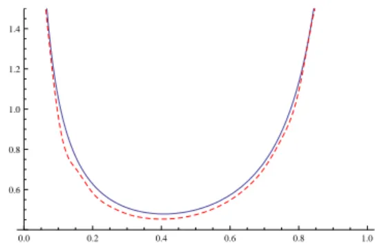
The Leading-Order Energy-Energy Correlation Function
- Structure of One-loop Amplitude in Four Dimension
- Calculation of Cut–constructible Contributions via Unitarity
- Box Integral coefficient
- Triangle Integral coefficient
- Bubble Integral coefficient
We would like to calculate the cut-constructible part of the amplitude Aone-loop MHV(φ,1,2,3). To calculate the cut-constructible part of the amplitude Aone-loop MHV(1,2,3), we should also sum over six unity cuts and suppress the overlapped loop integrals, we obtain the cut-constructible part of the amplitudeAone-loop MHV (1,2,3).

Rational part
Finally, we can have the cut-constructible part of all-negative helicity and MHV amplitudes Aone loop, CC(φ,1,2,3), in eq. 3.39) by summing the products of the basic integral and their coefficients obtained by the common unit method. We can also obtain the cut constructible part of all-positive helicity and MHV amplitudesAone loop, CC(φ†,1,2,3).
Calculations of the Virtual Contribution to the EEC Function
I proceed as follows: use a Mellin-Barnes representation of the integrand; perform phase-space integrals. In Section 4.7, I add up all the different parts of the real emission contribution to the energy–energy correlation and show that the divergent terms cancel against the virtual contribution (3.109).
Four-Particle Phase Space
For the other six integrals I obtain compact results for the divergent parts in ʻ, and series expansions of the finite part in ʻ. 4.4) Since we notice that there is a delta function δ(cosθij −c) in the integrand of the energy-energy correlation function, we want a parameterization that expresses cosθij as simply as possible, so that the delta function directly removes one integration.
Basic Integrals for the Energy-Energy Correlation
In the text below, I will calculate the dimensionless integral C8,a′ instead of C8,a, where C8,a′ is defined as,. where the general trivial factor 8 is just for simplicity and fdim was defined as follows,.
Mellin–Barnes representation for the Calculation of the Basic Integrals
A Shortcut
For example, if we integrate the variables13 with the parameterization (4.5), the arguments of the hypergeometric function are With these two steps, we can obtain a Mellin-Barnes Euclidean representation of the integrand containing the hypergeometric function (4.31).
Another Method to Compute the Coefficients of 1/ǫ 2 and 1/ǫ
For this and the entire Mellin-Barnes representation of the 1/ǫ2 and 1/ǫ coefficients of the basic integrals, we did not need to calculate the series expansion, but we perform the direct expansion of its Mellin-Barnes representation. But for some more complicated Mellin-Barnes representations, we will perform the substitution in Eq. 4.53) to calculate the inu series expansion.
Calculation of the Integral C 8,a ′
In this way we can directly find the compact analytical form of the expansion in| to acquire. However, for the integral C8,a we can obtain the coefficients analytically because the other integrals are simple.
Calculation of the Integral C 8,b ′
Finally, this leaves us with a series that is without lnuandπ:. 4.78) where the above basis function is chosen because it is the only combination involving Li3(1−u) that is without ζ3, lnuandπ. It is not complicated to repeat all the steps that were done for C8,a in the last subsection.
Calculations of the Integral C 8,d ′
We can use the same ansatz in the calculation of the integral C8,a so that we can fit the unknown coefficients in our ansatz. 4.95). Or we can use the following tricks to rewrite a one-dimensional integral into a summation of several one-dimensional integrals, so that we can apply the first Barnes lemma to each in that summation.
Calculation of the Integral C 8,e ′
Then we apply MBasymptotics to the coefficient ǫ0 to obtain its series coefficients for uk. We calculate series coefficients for uk to an order to compare with the approach to obtain the analytic form of the integral C8,e,.
Calculations of the Remaining Basic Integrals
4.108) On the integral IntEk we apply MBexpandin order to expand them to a series in ǫto ǫ0 order. The series coefficients of uk can be reduced to one-dimensional Mellin–Barnes integrals to which we can apply the Barnes lemmas.
Calculations of the Integral C 8,c ′
We use routine MBasymptotics for the coefficient ǫ0 to obtain the series expansion of inu. This way I can get the string expansion of atu= 1 and see if we can get more information about C8,c′.
Calculations of the integral C 8,f ′
During the evaluation of the coefficient ofu we will encounter some 3D Mellin-Barnes integrals such as:. We can calculate the series coefficients of u up to a high order of the coefficient of lnuinC8,f,0,lnu.
Calculations of the Integral C 8,g ′
3(1−u) (4.180) But in the end, even with an increased ansatz for fitting the series, I still fail to calculate its compact form.
Calculations of the Integral C 8,h ′
4.187) We then apply the MBexpand routine to each IntHk to expand the integrands into a series in the order ∫to ∫0. By following these procedures, all higher-dimensional Mellin-Barnes integrals can be reduced to one-dimensional ones.
Calculations of the integral C 8,i ′
Here we focus on the coefficient ofǫ0 obtained by applying the routineMBexpand to the sumP4. We can extract the coefficient ofǫ0 and we apply the routine MBasymptotics to it to obtain the series coefficients ofu.
Calculations of the Integral C 8,j ′
We apply the routineMBexpand to each integral in the sumP5. k=1IntLk to expand the integrands to series in the order up to 0. We apply the routineMBexpand to the sumP4. k=1IntMkin to obtain the 0order series coefficient.
Numerical Evaluations of all Base Integrals
When we evaluate CN,8,e,0′, we notice that there is a Mellin-Barnes integral M B7 which cannot be directly evaluated by MBintegration. In the numerical evaluation of CN,8,j,0′, we found a Mellin-Barnes integralM B8, which cannot be evaluated by integrating MB:.
The Calculation of the Definite Integral CL 3 (u)
Now we can apply the routine MBresolve to the above formula to solve its singularities and apply MBexpand to expand it as a series in ǫ. We can check numerically that the series expansion calculated by Mellin–Barnes representation is actually the series expansion of CL′3(u) nearu= 0.
Combining All Contributions
I will then show how to generalize the one-dimensional ansatz to two-dimensional Mellin–Barnes integrals. This ansatz should apply to both two-dimensional and higher-dimensional Mellin-Barnes integrals.
One-Dimensional Mellin–Barnes Integrals
A Euclidean integral with one stationary point in the fundamental region
We will not attempt to find the exact functional form for the stationary phase contour. The disappearance of the coefficient oft2 requires that d= 0 ifG′′(z0) does not vanish; d= 0 means that the tangent of the stationary phase contour atz0 is orthogonal to the real axis.

A Minkowski integral with a lone stationary point in the fundamental region
The value φ−∞ = π/2 means that the asymptotic stationary phase contour is parallel to the real axis. Finally, we glue the two parts of the contour together to obtain the full approximation to the stationary phase contour.

Integrands with two stationary points in the fundamental region
Whent→ ∞ we can guarantee the correct asymptotic behavior of the contour by using the ansatz, z(t) =z+∞+i teiφ∞+ whenℑz(t)>0,. Alternatively, we can shift the contour to a region where the integrand does not vanish, so that we can find a stationary point on the real axis.

Two-Dimensional Integrals
Parametrization of the 2-D Surface in Euclidean Case with one single stationary point
For the given example, there is a solitary stationary point which is also the minimum of the integrand in the fundamental region, so we do not need to shift the contour and calculate additional residuals. The choice made here allows us to analytically solve the unknown function Fs(θ) in the ansatz, when we have a single stationary point on the real cut in a fundamental region where the integral does not vanish generically .

Higher Dimension Euclidean Case with the extremum on the real slice
These requirements do not prevent their values, especially of the imaginary parts of z1±z2, from disappearing and thus ending up on a pole of a gamma function.
A First Minkowski Integral
If we calculate the intersection of our contour with the real slice, we can see that it is still in the fundamental region, so we don't need to shift the integral. We can evaluate the integral on this contour numerically and find that the result agrees with the evaluation on the naive contour.
A Second Minkowski Integral
For this given example, the intersection of the contour and the real slice is still in the original fundamental region. We can then use the contour to evaluate the integral numerically. 5.21 we present the values of the integrand on the found surface.

The Integrand with One PolyGamma Functions with Two Stationary Points in the Funda-
But in practice, for all the examples we investigated in this chapter, the contour avoids all singularities of the integrand and also leads to the correct result. In the following text we will try to find the contour of the stationary phase without moving the contour.

The integrand with several stationary points in the fundamental region
For the complex stationary points, the phase of the integrand at these suitable base points is all different. For each suitable base point, we can apply the ansatz (5.139) in last example to obtain a contour that yields the correct integral result.

Higher Dimension Case for both Euclidean and Minkowski integrals
We can apply the ansatz Eq. 5.139) at any convenient base point to obtain the contours and use these contours to evaluate the integral. The function φ∞(θ, φ) can be solved by the fact that we require that the argument of the asymptotic form of the integrand has no non-proportional tot term.