Fonctionnelles d’´energie non-empiriques pour la structure nucl´eaire

Common operators

Mathematical functions

• Clebsh-Gordan and Wigner coefficients
• Tensorial representations
• Spherical harmonics
• Tensor spherical harmonics
• Spherical Bessel functions
• Legendre polynomials
• Jacobi polynomials

A spherical tensor of rankl can be constructed from components of two other tensors, namely Tm[ℓ]= X. Standard spherical harmonics are defined as normalized eigenstates of angular momentum operators L2 and Lz. A.9) These functions have the following properties. The inverse relation for the expansion of the tensorial product of spherical harmonics is hY[ℓ1](ˆp)⊗Y[ℓ2](ˆp)i[ℓ]m.

Angular expansions

• Legendre polynomials expansion
• Dirac 3D delta function decomposition
• Polynomial decomposition
• Gaussian decomposition
• One-pion-exchange form factor decomposition

In this case, the form factors pf(~k,~k′) = q2 should be taken into account for the direct terms. The f = 1 block is irrelevant to the partial wave decomposition, while one takes in the thef = 0 block.

Reduced matrix elements

• General relations
• Exchange terms
• Reduced matrix elements of selected operators
• Tensorial product of spherical harmonics
• Quadratic terms
• Gaussian terms
• Representation
• Symmetries

The focus is placed on the connection between the so-called traditional and Russian representations in the case where time-reversal symmetry is not assumed. Thez signature relates, in the limiting case of an axially symmetric system, to the projection of orbital momentum mℓ and spin σ onto the z axis according to.

Two-body states

As previously stated, the basis will be split into two halves according to the z-signature quantum number, and the pairing is assumed to occur between states of opposite signature.

Time-reversal operator

• Definition
• Action on single-particle wave functions
• Transformation of creation and annihilation operators
• Action on one-body Dirac bras and kets
• Matrix representation

This is, for example, the case of the eigenbasis of the position, spin and isospin operators {ˆa†~rσq}. The representation of the same operator in Hilbert space ˆT is obtained by its action on a basis ket |~r σ qi and brah~r σ q|as.

Energy density functional formalism

Normal density matrix, pair density matrix and pairing tensor

In the so-called traditional representation of the HFB formalism, the pairing tensor is introduced. Rather, in the so-called Russian representation of the HFB formalism, the pair density is used, and it is defined as.

Generalized density matrices

Eq.(B.40) is the matrix representation of the definition of the pair density matrix in an arbitrary matrix through. This result provides an advantage for using the Russian representation in the case of time-varying invariant systems.

Hartree-Fock-Bogoliubov equations

Traditional representation

This means that the solution to the minimization problem is a basis that simultaneously diagonalizes Hq′ and Rq. Having these quasiparticle eigenstates at hand, the normal density matrix and the pairing tensor can be calculated as.

Russian representation

Note, however, that Eq.(B.70) demonstrates that quasiparticle wave functions in the Russian representation are not solutions of the HFB equations when time-reversal invariance is not assumed [6]. B.71), the Russian representation corresponds to representing the lower component of the quasiparticle wave functions in the basis constructed with the time-reversed modes of those used to express the upper component. Due to the properties of the M×M unit matrix G, the first M/2 components of Vq[˜ρ] now have an opposite signature to the first M/2 components of Uq[˜ρ].

Coordinate ⊗ spin ⊗ isospin space

The introduction of Dirac notations in the HFB formalism raises questions due to the use of particle and quasiparticle operators/states. For example, the matrix elements of the coupling field ∆q in coordinate space are usually defined by

Time-reversal invariant systems

• Basic properties
• Quasiparticle states
• Densities
• Fields
• HFB equations

The traditional HFB equations [6] can now be recovered from Eq. B.70) using the time-reversal invariance of the system. Independently of any single-particle representation, it is found that the HFB equations, in the Russian representation, take the form for time-varying invariant systems.

Canonical basis

• Bloch-Messiah-Zumino decomposition in the traditional representation
• General case
• BCS-like occupation numbers
• Time-reversal invariant systems

In the HFB formalism, states are not paired a priori as in the BCS approach, except for the fact that only states with opposite signatures are linked by the Bogoliubov transformation. In the HFB theory, explicit expressions of (uqµ2, vµq2) can be obtained by making use of the fact that the minimization principle amounts to the part of the Hamiltonian ˆH corresponding to two-quasiparticle excitations, i.e. B.124 , cancel.

Quasiparticle basis

Quasiparticle states

For time-reversal systems, it can therefore be useful to rearrange each pair of canonical states (µ,µ)˜ according to ηµ and not ζµ as is generally done. However, if the system is not time-reversal invariant, the definition of vqµ must be made in terms of ζµ.

Normal and pair density matrices, pairing tensor

Local normal and pair scalar densities

Spherical systems

• Basic properties
• Time-reversal symmetry
• Canonical basis
• Quasiparticle basis
• Local densities
• HFB equations

The quantum numberζµ is used to distinguish between the two halves of the base (ζµ>0 andζµ<0). These last relations prove that the upper and lower components of the quasiparticle wave functions are indeed eigenstates of (~Lˆ2,J~ˆ2,Jˆz) with eigenvalues ​​(ljm) and can be written as.

Infinite nuclear matter

• Basic properties
• Time-reversal symmetry
• Canonical basis
• Quasiparticle basis
• Densities
• Gap equation

B.135) where the third part Cq of the Bogoliubov transformation is trivial since one is dealing with a BCS approximation, i.e. In the present case, the only difference between traditional and Russian quasiparticles in INM is related to the spin part of the lower component. Although the spatial part of all wave functions of interest is explicitly known in the present case, one can re-express non-local densities given by Eq. B.162a,B.162b) in terms of the spatial parts of the quasiparticle wavefunctions, that is.

Application to the bilinear EDF

• Basis sets for the N-body problem
• Decomposition of the N -body wave function
• Spectroscopic quantities
• Properties of the norm kernel N (i~r, j~r ′ )
• Coupled equations for the overlap functions
• Approximate decoupling of the problem
• Asymptotic behavior of the expansion coefficients

1All spin and isospin dependence of the N-body wave function cancel out here, and HN(~r1. Only the first term in the expansion of the input channel|Ψ~Nj thus contributes significantly to the total matrix element. On the other side Using the definition of C.6)), the core can be expressed in terms of the (N−1)-body overlap functions as.

Center-of-mass correlations

• Internal N -body wave function
• Decomposition of the N -body wave function
• Internal spectroscopic factors
• Coupled equations for the internal spectroscopic amplitudes
• Koltun sum rules
• Self-consistent translationally invariant theories
• Internal Slater determinants

N K~N −K~N−12 and is the Fourier transform of the intrinsic spectroscopic amplitude, which can be defined by removing from Eq. C.73) contribution of the center of mass, i.e. C.75b). It should be noted that the individual (intrinsic) spectroscopic factors can be greater than one for fermionic systems due to the motion of the center of mass. In order to prove that this breakdown in terms of relative motion with respect to the system of (N −1) bodies is the most accurate, it is possible to derive the equations satisfied by the amplitudes φi.

One-body density

Laboratory frame

However, it gives us a good insight into how the one-body density operator behaves. Using a trivial variable change, we find that the density of a body is invariant under any translation. Indeed, using Eq.(C.116), the density matrix in the laboratory frame is the sum of the spectroscopic amplitudes ˘ϕN0i in the same frame, i.e.

Internal density

To find the definition of the internal density operator in the full Hilbert space, Eq. (C.136) is generalized into. More generally, for an arbitrary translation of the center of mass of the system, one has ˆ. According to the coupled equation for the internal overlap function (Eq. C.97)) one finds that the asymptotics of the internal one-body density reads(18).

Energy density functional framework

Possible extensions

Tensor interaction

One-pion exchange interaction and Yukawa potential

The Hamiltonian of the meson field can be cast in a superposition of harmonic oscillators of energy ωq and coordinates kq. The Fourier transform gives the interaction in coordinate space in the form of the well-known Yukawa potential. In the low energy limit, the long-range part of the vacuum nucleon-nucleon interaction in the meson exchange model is dominated by the exchange of the lightest strongly interacting particle, known to be the pion.

Properties of the tensor operator

Therefore, for the action of spin point gradient operators on the Yukawa potential one gets ~σ1·∇~ ~σ2·∇~ e−µr.

Partial wave expansion

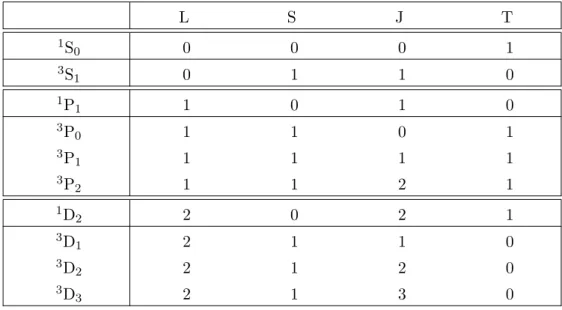
One is left with the elements of a partial wave matrix of the type vJSTLL′ (k, k′), with the conventions from Eqs. A.1b,A.1c), which are called interaction matrix elements in a given partial wave. Tzi, the interaction can be separated into isospin delvT and angular momentum vJ, and. D.41) Thus standard or reduced interaction matrix elements can be evaluated, which is easiest. Indeed, according to our conventions, the partial wave expansion of the Dirac delta 3D function (equation (A.52)) reads

Scattering phase shifts

Uncoupled channels

The SLJST restriction of the scattering matrix to the uncoupled channel is a scalar, and the scattered wave can be written as 26], the relation between the scattering phase shifts and the T-matrix for uncoupled channels is obtained by the following procedure. For very large distances r > R, the asymptotic solutions of equations (D.59a, D.59b) can be used, while the fully embedded T-matrix, expressed in units of fm, is restored on the right-hand side.

Uncoupled channels: alternate method

Using an integration of parts, we obtain D.64) For very large distances r > R, the asymptotic solutions from Eqs.(D.59a,D.59b) can be used, whereas the complete on-shellT matrix, expressed in fm units, is recovered in the right-hand side. Non-vanishing matrix elements for the latter expression can be obtained on the energy shell using Tab+ ≡ −2π i δ(Ea−Eb)Tab+, Tab ≡2π δ(Ea−Eb)Tab. 3 Strictly speaking, the T-matrix as defined by Lippmann and Schwinger is T+, while the T-matrix defined at the level of Eq.(D.48) is usually called the reactanceK matrix.

Coupled channels

The scattering phase shifts can be given either as a function of the relative momentum k or of the energy in the Elab laboratory frame, which reads Various formulations of the phase shifts in the presence of electromagnetic interaction are then possible, corresponding to a series of functions used to asymptotically match the interacting and non-interacting scattering solutions. They correspond to the notation δYX, which denotes the phase lag solution with potential X with respect to the asymptotic solution of potential Y.

Nuclear matter equation of state

• Kinetic energy
• Correlation energy at the Hartree-Fock level: generalities
• Correlation energy at the Hartree-Fock level: partial wave expansion
• Correlation energy at the Hartree-Fock evel: gaussian vertices
• Equivalence between the two methods
• Conventions and preliminary remarks
• Gogny interaction
• Microscopic vertex
• Tensor terms

Such a discharge uses a partial wave expansion of the vertex and thus consists of a converging series. The correlation energy of spin-unpolarized INM is read at the Hartree-Fock level as a double trace over the closed loops of the two-body potential TV, i.e. D.121b). In the case of infinite nuclear matter, the coupling constant is therefore independent of the center of mass position.

Partial wave expansion

D1X/D2 interaction

For reference, we provide a partial wave decomposition of the one-pawn exchange, whose corresponding vertex is in momentum space. 2This justifies the use of the function Θ in the expression offKσ, which Kas defines the maximum range of the smoothing. The generalization of the previous algorithm for the two-dimensional case, after removing all biases, is easy to read.

Unimodal functions

To evaluate the performance of the simplex and fitpack algorithms, several cost functions have been considered [55], corresponding to different situations in terms of (i) the existence of secondary minima (multimodal functions), (ii) the smoothness of the surface of the cost around the global minimum and (iii) dimensionality. We also suggest values ​​for the initial search space that are large enough to capture the complexity of the problem. Due to the nonlinearity of the valley, many algorithms converge slowly because they change the search direction repeatedly.

Multimodal functions with many local optima

Multimodal functions with few local optima

Random surface generator

One-dimension case

While the first three situations investigate different regimes of the algorithm, the last one allows to calculate the distribution of R(Xi) for each i. This undesirable property corresponds to the fact that β is statistically more likely to reach βmax at the problem's limits where only one half of the network is fully weighted by the effective area function fKσ. Only values ​​between the blue lines are actually considered at the end, other bins are only intermediate stages of the generator.

Two-dimension case

• Transformation rules
• Specific values
• P σ/τ operator
• Q
• Total angular momentum L
• h
• Spherical harmonics

Chersonsky: Quantum Theory of Angular Momentum: Irreducible Tensors, Spherical Harmonics, Vector Coupling Coefficients, 3NJ Symbols (World Scientific, Singapore, 1988). Mavrommatis: The one-body and two-body density matrices of finite nuclei with an appropriate treatment of the center-of-mass motion. Wagner: Is there evidence of three-body forces violating the Koltun energy sum rule.