Learning the Structure of Linear Latent Variable Models
Ricardo Silva [email protected]
Center for Automated Learning and Discovery School of Computer Science
Richard Scheines [email protected]
Clark Glymour [email protected]
Peter Spirtes [email protected]
Department of Philosophy Carnegie Mellon University Pittsburgh, PA 15213, USA
Editor:XXX
Abstract
We describe anytime search procedures that (1) find disjoint subsets of recorded variables for which the members of each subset are d-separated by a single common unrecorded cause, if such exists; (2) return information about the causal relations among the latent factors so identified. We prove the procedure is point-wise consistent assuming (a) the causal relations can be represented by a directed acyclic graph (DAG) satisfying the Markov Assumption and the Faithfulness Assumption; (b) unrecorded variables are not caused by recorded variables; and (c) dependencies are linear. We compare the procedure with factor analysis over a variety of simulated structures and sample sizes, and illustrate its practical value with brief studies of social science data sets. Finally, we consider generalizations for non-linear systems.
Keywords: Latent variable models, causality, graphical models, structural equation models
1. What we will show
In many empirical studies that estimate causal relationships, influential variables are un- recorded, or “latent.” When unrecorded variables are believed to influence only one recorded variable directly, they are commonly modeled as noise. When, however, they influence two or more measured variables directly, the intent of such studies is to identify them and their influences. In many cases, for example in sociology, social psychology, neuropsychology, epidemiology, climate research, signal source studies, and elsewhere, the chief aim of in- quiry is in fact to identify the causal relations of (often unknown) unrecorded variables that influence multiple recorded variables. It is often assumed on good grounds that recorded variables do not influence unrecorded variables, although in some cases recorded variables may influence one another.
When there is uncertainty about the number of latent variables, which measured vari- ables they influence, or which measured variables influence other measured variables, the investigator who aims at a causal explanation is faced with a difficult discovery problem for which currently available methods are at best heuristic. Loehlin (2004) argues that while there are several approaches to automatically learn causal structure, none can be seem as competitors of exploratory factor analysis: the usual focus of automated search proce- dures for causal Bayes nets is on relations among observed variables. Loehlin’s comment overlooks Bayes net search procedures robust to latent variables (Spirtes et al., 2000), but the general sense of his comment is correct. For a kind of model widely used in applied sciences − “multiple indicator models” in which multiple observed measures are assumed to be effects of unrecorded variables and possibly of each other − machine learning has provided no principled alternative to factor analysis, principal components, and regression analysis of proxy scores formed from averages or weighted averages of measured variables, the techniques most commonly used to estimate the existence and influences of variables that are unrecorded. The statistical properties of models produced by these methods are well understood, but there are no proofs, under any general assumptions, of convergence to features of the true causal structure. The few simulation studies of the accuracy of these methods on finite samples with diverse causal structures are not reassuring (Glymour, 1997).
The use of proxy scores with regression is demonstrably not consistent, and systematically overestimates dependencies. Better methods are needed.
We describe a two part method for this problem. The method (1) finds clusters of measured variables that are d-separated by a single unrecorded common cause, if such exists; and (2) finds features of the Markov Equivalence class of causal models for the latent variables. Assuming only principles standard in Bayes net search algorithms, and satisfied in almost all social science models, the two procedures converge, probability 1 in the large sample limit, to correct information. The completeness of the information obtained about latent structure depends on how thoroughly confounded the measured variables are, but when, for each unknown latent variable, there in fact exists at least a small number of measured variables that are influenced only by that latent variable, the method returns the complete Markov Equivalence class of the latent structure. We show by simulation studies for three latent structures and for a range of sample sizes that the method identifies the number of latent variables more accurately than does factor analysis. Applying the search procedures for latent structure to the latent variables identified (1) by factor analysis and, alternatively, (2) by our clustering method, we again show by simulation that our clustering procedure is more accurate. We illustrate the procedure with applications to social science cases.
2. Illustrative principles
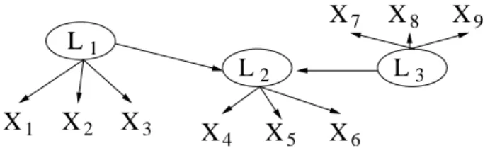
Consider Figure 1, whereXvariables are recorded andLvariables (in ovals) are unrecorded and unknown to the investigator.
The latent structure, the dependencies of measured variables on individual latent vari- ables, and the linear dependency of the measured variables on their parents and (unrepre- sented) independent noises in Figure 1 imply a pattern of constraints on the covariance ma- trix among theXvariables. For example,X1, X2, X3have zero covariances withX7, X8, X9.
3 2 X3
X9 X7 X8
X6 X5 L2
X1 X4
L1
L X
Figure 1: A latent variable model which entails several constraints on the observed covari- ance matrix. Latent variables are inside ovals.
Less obviously, forX1, X2, X3 and any one ofX4, X5, X6, three quadratic constraints (tetrad constraints) on the covariance matrix are implied: e.g., forX4
ρ12ρ34=ρ14ρ23=ρ13ρ24 (1) whereρ12 is the Pearson product moment correlation betweenX1, X2, etc. (Note that any two of the three vanishing tetrad differences above entails the third.) The same is true for X7, X8, X9 and any one of X4, X5, X6; for X4, X5, X6, and any one of X1, X2, X3 or any one of X7, X8, X9. Further, for any two of X1, X2, X3 or of X7, X8, X9 and any two of X4, X5, X6, exactly one such quadratic constraint is implied, e.g., for X1, X2 and X4, X5, the single constraint
ρ14ρ25=ρ15ρ24 (2)
The constraints hold as well if covariances are substituted for correlations.
Statistical tests for vanishing tetrad differences are available for a wide family of distrib- utions. Linear and non-linear models can imply other constraints on the correlation matrix, but general, feasible computational procedures to determine arbitrary constraints are not available (Geiger and Meek, 1999) nor are there any available statistical tests of good power for higher order constraints.
Given a “pure” set of sets of measured indicators of latent variables, as in Figure 1
− informally, a measurement model specifying, for each latent variable, a set of measured variables influenced only by that latent variable and individual, independent noises −the causal structure among the latent variables can be estimated by any of a variety of methods.
Standard chi square tests of latent variable models can be used to compare models with and without a specified edge, providing indirect tests of conditional independence among latent variables. The conditional independence facts can then be input to a constraint based Bayes net search algorithm, such as PC or FCI (Spirtes et al., 2000). Such procedures are asymptotically consistent, but not necessarily optimal on small samples. Alternatively, a correlation matrix among the latent variables can be estimated from the measurement model and the correlations among the measured variables, and a Bayesian search can be used. Score-based approaches for learning the structure of Bayesian networks, such as GES (Chickering, 2002), are usually more accurate with small to medium sized samples than are PC or FCI. Given an identification of the latent variables and a set of “pure” measured effects or indicators of each latent, the correlation matrix among the latent variables can be estimated by expectation maximization, The complete graph on the latent variables is then
3 2 X3
X9 X7 X8
X6 X5 X4
L4 X10 X11 X12 X13 L2
X1 L1
L X
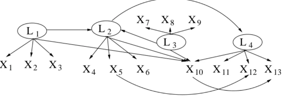
Figure 2: A latent variable model which entails several constraints on the observed covari- ance matrix.
dispensed with and the latent structure is estimated from the estimated correlations, using GES with the Bayes Information Criterion (BIC) score to estimate posterior probabilities.
In Figure 1 the measured variables neatly cluster into disjoint sets of variables and the variables in any one set are influenced only by a single common cause and there are no influences of the measured variables on one another. In many real cases the influences on the measured variables do not separate so simply. Some of the measured variables may influence others (as in signal leakage between channels in spectral measurements), and some or many measured variables may be influenced by two or more latent variables.
For example, the latent structure of a linear, Gaussian system shown in Figure 2 can be recovered by the procedures we propose. Our aim in what follows is to prove and use new results about implied constraints on the covariance matrix of measured variables to form measurement models that enable estimation of features of the Markov Equivalence class of the latent structure in a wide range of cases. We will develop the theory first for linear models with a joint Gaussian distribution on all variables, including latent variables, and then consider possibilities for generalization. In many models of this kind in the applied sciences, some variables are specified with unexplained correlations represented as bidirected edges between the variables. We allow representations of this kind.
The general idea is as follows. We introduce a graphical representation of an equivalence class of models that entail a given set of vanishing partial correlations and vanishing tetrad differences, analogous to the familiar notion of a pattern (Pearl, 1988) used to represent a Markov Equivalence class of directed acyclic graphs (DAGs), We provide an algorithm for discovering features of this Measurement Pattern. Using the Measurement Pattern, further procedures find clusters of measured variables for which the members of each cluster share a latent common cause. A combination of expectation-maximization and the GES algorithm scored by BIC is then used to estimate the causal relations among the latent variables.
3. Related work
The traditional framework for discovering latent variables is factor analysis and its variants (see, e.g., Bartholomew et al., 2002). A number of factors is chosen based on some criterion such as the minimum number of factors that fit the data at a given significance level or
the number that maximizes a score such as BIC. After fitting the data, usually assuming a Gaussian distribution, different transformations (rotations) to the latent covariance matrix are applied in order to satisfy some criteria of simplicity. Latents are interpreted based on the magnitude of the coefficients relating each observed variable to each latent.
In non-Gaussian cases, the usual methods are variations of independent component analysis, such as independent factor analysis (Attias, 1999) and tree-based component analysis (Bach and Jordan, 2003). These methods severely constrain dependency struc- ture among the latent variables. That facilitates joint density estimation or blind source separation, but it is of little use in learning causal structure.
In a similar vein, Zhang (2004) represents latent variable models for discrete variables (both observed and latent) with a multinomial probabilistic model. The model is con- strained to be a tree and every observed variable has one and only one (latent) parent and no child. Zhang does not provide a search method to find variables satisfying the assumption, but assumes a priori the variables measured satisfy it.
Elidan et al. (2000) introduces latent variables as common causes of densely connected regions of a DAG learned through standard algorithms for learning Bayesian network struc- tures. Once one latent is introduced as the parent of a set of nodes originally strongly connected, the standard search is executed again. The process can be iterated to intro- duce multiple latents. Examples are given for which this procedure increases the fit over a latent-free graphical model are provided, but Elidan et al. provide no information about the conditions under which the estimated causal structure is correct. In Silva et al. (2003) we developed an approach to learning measurement models. That procedure requires that the true underlying graph has a “pure” submodel with three measures for each latent variable, which is a strong and generally untestable assumption. That assumption is not needed in the procedures described here.
4. Notation, assumptions and definitions
Our work is in the framework of causal graphical models. Concepts used here without explicit definition, such as d-separation and I-map, can be found in standard sources (Pearl, 1988; Spirtes et al., 2000; Pearl, 2000). We use “variable” and “vertex” interchangeably, and standard kinship terminology (“parent,” “child,” “descendant,” “ancestor”) for directed graph relationships. Sets of variables are represented in bold, individual variables and symbols for graphs in italics. The Pearson partial correlation of X,Y controlling for Z is denoted by ρXY.Z. We assume i.i.d. data sampled from a subset O of the variables of a joint Normal distributionDon variablesV=O∪L, subject to the following assumptions:
A1 Dfactors according to the local Markov assumption for a DAG Gwith vertex set V.
That is, any variable is independent of its non-descendants in G conditional on any values of its parents inG.
A2 No vertex inO is an ancestor of any vertex in L. We call this property the measure- ment assumption;
A3 Each variable in V is a linear function of its parents plus an additive error term of positive finite variance
A4 The Faithfulness Assumption: for all {X, Y, Z} ⊆ V, X is independent of Y condi- tional on each assignment of values to variables inZ if and only if the Markov Assump- tion forGentails such conditional independencies. For models satisfying A1-A3 with Gaussian distributions, Faithfulness is equivalent to assuming that no correlations or partial correlations vanish because of multiple pathways whose influences perfectly cancel one another.
Definition 1 (Linear latent variable model) A model satisfying A1 − A4 is a linear latent variable model, or for brevity, where the context makes the linearity assumption clear, a latent variable model.
A single symbol, such as G, will be used to denote both a linear latent variable model and the corresponding latent variable graph. Linear latent variable models are ubiquitous in econometric, psychometric, and social scientific studies (Bollen, 1989), where they are usually known as structural equation models.
Definition 2 (Measurement model) Given a linear latent variable modelG, with vertex set V, the subgraph containing all vertices inV, and all and only those edges directed into vertices in O, is called the measurement model of G.
Definition 3 (Structural model) Given a linear latent variable model G, the subgraph containing all and only its latent nodes and respective edges is the structural model of G.
Definition 4 (Linear entailment) We say that a DAGG linearly entails a constraint if and only if the constraint holds in every distribution satisfying A1 - A4 forGwith covariance matrix parameterized by Θ, the set of linear coefficients and error variances that defines the conditional expectation and variance of a vertex given its parents.
Definition 5 (Tetrad equivalence class) Given a setCof vanishing partial correlations and vanishing tetrad differences, a tetrad equivalence classT(C)is the set of all latent vari- able graphs each member of which entails all and only the tetrad constraints and vanishing partial correlations among the measured variables entailed by C.
Definition 6 (Measurement equivalence class) An equivalence class of measurement models M(C) forCis the union of the measurement models graphs inT(C). We introduce a graphical representation of common features of all elements of M(C), analogous to the familiar notion of a pattern representing the Markov Equivalence class of a Bayes net.
Definition 7 (Measurement pattern) A measurement pattern, denoted MP(C), is a graph representing features of the equivalence class M(C) satisfying the following:
• there are latent and observed vertices;
• the only edges allowed in an MP are directed edges from latent variables to observed variables, and undirected edges between observed vertices;
• every observed variable in a MP has at least one latent parent;
Algorithm FindPattern Input: a covariance matrix Σ
1. Start with a complete graphGover the observed variables.
2. Remove edges for pairs that are marginally uncorrelated or uncorrelated conditioned on a third variable.
3. For every pair of nodes linked by an edge in G, test if some rule CS1, CS2 or CS3 applies. Remove an edge between every pair corresponding to a rule that applies.
4. LetH be a graph with no edges and with nodes corresponding to the observed vari- ables.
5. For each maximal clique in G, add a new latent to H and make it a parent to all corresponding nodes in the clique.
6. For each pair (A, B), if there is no other pair (C, D) such thatσACσBD =σADσBC = σABσCD, add an undirected edgeA−B to H.
7. Return H.
Table 1: Returns a measurement pattern corresponding to the tetrad and first order van- ishing partial correlations of Σ.
• if two observed variablesX andY in aMP(C) do not share a common latent parent, then X and Y do not share a common latent parent in any member ofM(C);
• if observed variables X and Y are not linked by an undirected edge in MP(C), then X is not an ancestor of Y in any member of M(C).
Definition 8 (Pure measurement model) A pure measurement model is a measure- ment model in which each observed variable has only one latent parent, and no observed parent. That is, it is a tree beneath the latents.
5. Procedures for finding pure measurement models
Our goal is to find pure measurement models whenever possible, and use them to estimate the structural model. To do so, we first use properties relating graphical structure and covariance constraints to identify a measurement pattern, and then turn the measurement pattern into a pure measurement model.
FindPattern, given in Table 1, is an algorithm to learn a measurement pattern from an oracle for vanishing partial correlations and vanishing tetrad differences. The algorithm uses three rules, CS1, CS2, CS3, based on Lemmas that follow, for determining graphical structure from constraints on the correlation matrix of observed variables.
Let C be a set of linearly entailed constraints that exist in the observed covariance matrix. The first stage of FindPattern searches for subsets of C that will guarantee
X1 X2 Y
1 Y
Y 3 3 2
X X1 Y
1 Y
Y 3 3 2
X2 X
X
Y
X1 X2 Y
1 Y
Y 3 3 2
X
(a) (b) (c)
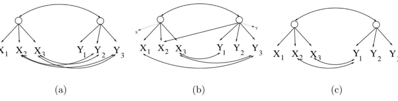
Figure 3: Three examples with two main latents and several independent latent common causes of two indicators (represented by double-directed edges). In (a), CS1 applies, but not CS2 nor CS3 (even when exchanging labels of the variables); In (b), CS2 applies (assuming the conditions for X1, X2 and Y1, Y2), but not CS1 nor CS3. In (c), CS3 applies, but not CS1 nor CS2.
that two observed variables do not have any latent parent in common. LetG be the latent variable graph for a linear latent variable model with a set of observed variablesO. LetO′= {X1, X2, X3, Y1, Y2, Y3} ⊂Osuch that for all triplets{A, B, C},{A, B} ⊂O′andC∈O, we have ρAB 6= 0, ρAB.C 6= 0. LetτIJ KL represent the tetrad constraintσIJσKL−σIKσJ L = 0 and ¬τIJ KL represent the complementary constraintσIJσKL−σIKσJ L6= 0:
Lemma 9 (CS1 Test) If constraints{τX1Y1X2X3, τX1Y1X3X2, τY1X1Y2Y3, τY1X1Y3Y2,¬τX1X2Y2Y1} all hold, then X1 andY1 do not have a common parent inG.
“CS” here stands for “constraint set,” the premises of a rule that can be used to test if two nodes do not share a common parent. Other sets of observable constraints can be used to reach the same conclusion.
Let the predicate F1(X, Y, G) be true if and only if there exist two nodes W and Z in latent variable graph G such that τW XY Z and τW XZY are both linearly entailed by G, all variables in {W, X, Y, Z} are correlated, and there is no observed C in G such that ρAB.C = 0 for{A, B} ⊂ {W, X, Y, Z}:
Lemma 10 (CS2 Test) If constraints {τX1Y1Y2X2, τX2Y1Y3Y2, τX1X2Y2X3,¬τX1X2Y2Y1} all hold such that F1(X1, X2, G) =true, F1(Y1, Y2, G) =true, X1 is not an ancestor of X3 and Y1 is not an ancestor of Y3, then X1 and Y1 do not have a common parent in G.
Lemma 11 (CS3 Test) If constraints{τX1Y1Y2Y3, τX1Y1Y3Y2, τX1Y2X2X3, τX1Y2X3X2, τX1Y3X2X3, τX1Y3X3X2, ¬τX1X2Y2Y3} all hold, then X1 and Y1 do not have a common parent in G.
These rules are illustrated in Figure 3. The rules are not redundant: only one can be applied on each situation. For CS2 (Figure 3(b)), nodesX and Y are depicted as auxiliary nodes that can be used to verify predicates F1. For instance, F1(X1, X2, G) is true because all three tetrads in the covariance matrix of{X1, X2, X3, X} hold.
Sometime it is possible to guarantee that a node is not an ancestor of another, as required, e.g., to apply CS2:
X X2 X3 X4 X5 X6 8
X X7
1 X 8
X6
X5
X4
X2
X7
X3 X
1
(a) (b)
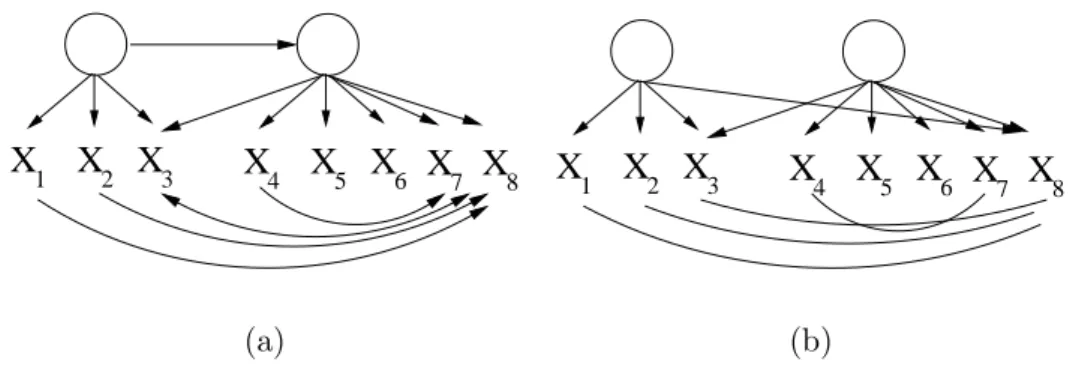
Figure 4: In (a), a model that generates a covariance matrix Σ. In (b), the output of FindPatterngiven Σ. Pairs in{X1, X2} × {X4, . . . , X7} are separated by CS2.
Lemma 12 If for some set O′ = {X1, X2, X3, X4} ⊆ O, σX1X2σX3X4 = σX1X3σX2X4 = σX1X4σX2X3 and for all triplets {A, B, C}, {A, B} ⊂ O′, C ∈ O, we have ρAB.C 6= 0 and ρAB 6= 0, then A∈O′ is not a descendant in Gof any element of O′\{A}.
For instance, in Figure 3(b) the existence of the observed node X (linked by a dashed edge to the parent of X1) allows the inference that X1 is not an ancestor of X3, since all three tetrad constraints hold in the covariance matrix of{X, X1, X2, X3}.
Theorem 13 The output ofFindPatternis a measurement pattern MP(C) with respect to the tetrad and zero/first order vanishing partial correlation constraints C of Σ.
The presence of an undirected edge does not mean that adjacent vertices in the pattern are actually adjacent in the true graph. Figure 4 illustrates this: X3andX8share a common parent in the true graph, but are not adjacent. Observed variables adjacent in the output pattern always share at least one parent in the pattern, but do not always share a common parent in the true DAG. Vertices sharing a common parent in the pattern might not share a parent in the true graph (e.g.,X1 and X8 in Figure 4 ).
The FindPattern algorithm is sound, but not necessarily complete. That is, there might be graphical features shared by all members of the measurement model equivalence class that are not discovered by FindPattern. Using the notion of a pure measurement model, defined above, we can improve the results with respect to a subset of the given variables. A pure measurement model implies a clustering of observed variables: each cluster is a set of observed variables that share a common (latent) parent, and the set of latents defines a partition over the observed variables. The output of FindPattern cannot, however, reliably be turned into a pure measurement pattern in the obvious way, by removing fromH all nodes that have more than one latent parent and one of every pair of adjacent nodes.
The procedureBuildPureClustersof Table 2 builds a pure measurement model using FindPattern and an oracle for constraints as input. Variables are removed whenever appropriate tetrad constraints are not satisfied. Some extra adjustments concern clusters
with proper subsets that are not consistently correlated to another variable (Steps 6 and 7) and a final merging of clusters (Step 8). We explain the necessity of these steps in Appendix A. As described, BuildPureClusters requires some decisions that are not specified (Steps 2, 4, 5 and 9). We propose an implementation in Appendix C, but various results are indifferent to how these choices are made.
The graphical properties of the output ofBuildPureClustersare summarized by the following theorem:
Theorem 14 Given a covariance matrix Σ assumed to be generated from a linear latent variable model G with observed variables O and latent variables L, let Gout be the output of BuildPureClusters(Σ) with observed variables Oout ⊆O and latent variables Lout. ThenGout is a measurement pattern, and there is an unique injective mappingM :Lout → L with the following properties:
1. Let Lout∈Lout. LetX be a child ofLout in Gout. ThenM(Lout) d-separates X from Oout\X in G;
2. M(Lout) d-separates X from every latent L in G for which M−1(L) is defined;
3. Let O′ ⊆Oout be such that each pair in O′ is correlated. At most one element in O′ has the following property: (i) it is not a descendant of its respective mapped latent parent in G or (ii) it has a hidden common cause with its respective mapped latent parent in G;
Informally, there is a labeling of latents in Gout according to the latents inG, and in this relabeled output graph any d-separation between a measured node and some other node will hold in the true graph, G. For each group of correlated observed variables, we can guaranteee that at most one edge from a latent into an observed variable is incorrectly directed. Notice that we cannot guarantee that an observed nodeXwith latent parentLout inGout will be d-separated from the other nodes in Ggiven M(Lout): if X has a common cause with M(Lout), then X will be d-connected to any ancestor of M(Lout) in G given M(Lout).
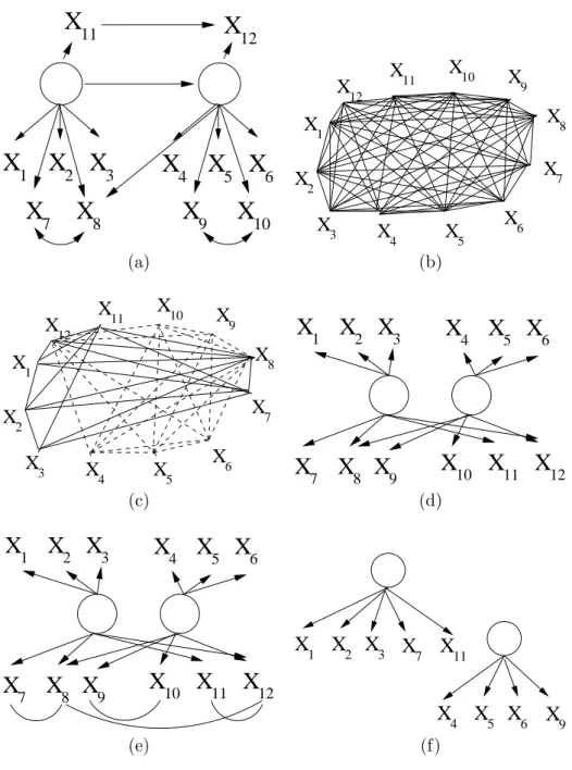
To illustrate BuildPureClusters, suppose the true graph is the one given in Fig- ure 5(a), with two unlabeled latents and 12 observed variables. This graph is unknown to BuildPureClusters, which is given only the covariance matrix of variables{X1, X2, ..., X12}.
The task is to learn a measurement pattern, and then a purified measurement model.
In the first stage of BuildPureClusters, theFindPatternalgorithm, we start with a fully connected graph among the observed variables (Figure 5(b)), and then proceed to remove edges according to rules CS1, CS2 and CS3, giving the graph shown in Figure 5(c). There are two maximal cliques in this graph: {X1, X2, X3, X7, X8, X11, X12} and {X4, X5, X6, X8, X9, X10, X12}. They are distinguished in the figure by different edge rep- resentations (dashed and solid - with the edgeX8−X12 present in both cliques). The next stage takes these maximal cliques and creates an intermediate graphical representation, as depicted in Figure 5(d). In Figure 5(e), we add the undirected edges X7−X8,X8−X12, X9−X10 and X11−X12, finalizing the measurement pattern returned by FindPattern.
Finally, Figure 5(f) represents a possible purified output ofBuildPureClustersgiven this
Algorithm BuildPureClusters Input: a covariance matrix Σ
1. G←FindPattern(Σ).
2. Choosea set of latents inG. Remove all other latents and all observed nodes that are not children of the remaining latents and all clusters of size 1.
3. Remove all nodes that have more than one latent parent in G.
4. For all pairs of nodes linked by an undirected edge, choose one element of each pair to be removed.
5. If for some set of nodes {A, B, C}, all children of the same latent, there is a fourth node D in G such that σABσCD = σACσBD = σADσBC is not true, remove one of these four nodes.
6. For every latent L with at least two children, {A, B}, if there is some node C in G such thatσAC = 0 andσBC 6= 0, splitLinto two latentsL1 andL2, whereL1becomes the only parent of all children of L that are correlated with C, and L2 becomes the only parent of all children of Lthat are not correlated with C;
7. Remove any cluster with exactly 3 variables {X1, X2, X3} such that there is no X4 where all three tetrads in the covariance matrixX={X1, X2, X3, X4} hold, all vari- ables ofX are correlated and no partial correlation of a pair of elements of Xis zero conditioned on some observed variable;
8. While there is a pair of clusters with latents Li and Lj, such that for all subsets {A, B, C, D} of the union of the children of Li, Lj we have σABσCD = σACσBD = σADσBC, and no marginal independence or conditional independence in sets of size 1 are observed in this cluster, set Li=Lj (i.e., merge the clusters);
9. Again, verify all implied tetrad constraints and remove elements accordingly. Iterate with the previous step till no changes happen;
10. Remove all latents with less than three children, and their respective measures;
11. ifGhas at least four observed variables, returnG. Otherwise, return an empty model.
Table 2: A general strategy to find a pure MP that is also a linear measurement model of a subset of the latents in the true graph. As explained in the body of the text, steps 2, 4, 5 and 9 are not described algorithmically in this Section.
12
X X
6X
5X
4X
2X
3X X
X X X X
7 8 9 10
11
1
X
X4
X5 X6 X7
X9
X2
X1
X12
X8
X11 X10
3
(a) (b)
X
X4 X5 X6 X7
X9
X2
X1
X12
X8 X11 X
10
3
X X
2X
3X
6X
5X
4X
7X
8X
9X
10X
11X
121
(c) (d)
X X
2X
3X
6X
5X
4X
7X
8X
9X
10X
11X
121
X X2 X3 X7 X11
X6
X5
X4 X9
1
(e) (f)
Figure 5: A step-by-step demonstration of how a covariance matrix generated by graph in Figure (a) will induce the pure measurement model in Figure (f).
pattern. Another purification with as many nodes as in the graph in Figure 5(f) substitutes node X9 for nodeX10.
The following result is essential to provide an algorithm that is guaranteed to find a Markov equivalence class for the latents inM(Lout) using the output of BuildPureClus- ters as a starting point:
Theorem 15 LetM(Lout)⊆Lbe the set of latents inGobtained by the mapping function M(). Let ΣOout be the population covariance matrix of Oout. Let the DAG Gaugout be Gout
augmented by connecting the elements of Lout such that the structural model of Gaugout is an I-map of the distribution of M(Lout). Then there exists a linear latent variable model usingGaugout as the graphical structure such that the implied covariance matrix of Oout equals ΣOout.
A further reason why we do not provide details of some steps ofBuildPureClustersat this point is because there is no unique way of implementing it, and different purifications might be of interest. For instance, one might be interested in the pure model that has the largest possible number of latents. Another one might be interested in the model with the largest number of observed variables. However, some of these criteria might be computationally intractable to achieve. Consider for instance the following criterion, which we denote as MP3: given a measurement pattern, decide if there is some choice of nodes to be removed such that the resulting graph is a pure measurement model and each latent has at least three children. This problem is intractable:
Theorem 16 Problem MP3 is NP-complete.
There is no need to solve a NP-hard problem in order to have the theoretical guarantees of interpretability of the output given by Theorem 14. For example, there is a stage in FindPatternwhere it appears necessary to find all maximal cliques, but, in fact, it is not.
Identifying more cliques increases the chance of having a larger output (which is good) by the end of the algorithm, but it is not required for the algorithms correctness. Stopping at Step 5 ofFindPattern before completion will not affect Theorems 14 or 15.
Another computational concern is the O(N5) loops in Step 3 of FindPattern, where N is the number of observed variables. Again, it is not necessary to compute this loop entirely. One can stop Step 3 at any time at the price of losing information, but not the theoretical guarantees ofBuildPureClusters. This anytime property is summarized by the following corollary:
Corollary 17 The output of BuildPureClustersretains its guarantees even when rules CS1, CS2 and CS3 are applied an arbitrary number of times in FindPattern for any arbitrary subset of nodes and an arbitrary number of maximal cliques is found.
6. Learning the structure of the unobserved
The real motivation for finding a pure measurement model is to obtain reliable statistical access to the relations among the latent variables. Given a pure and correct measurement model, even one involving a fairly small subset of the original measured variables, a variety of algorithms exist for finding a Markov equivalence class of graphs over the set of latents in the given measurement model.
6.1 Constraint-based search
Constraint based search algorithms rely on decisions about independence and conditional independence among a set of variables to find the Markov equivalence class over these
variables. Given a pure and correct measurement model involving at least 2 measures per latent, we can test for independence and conditional independence among the latents, and thus search for equivalence classes of structural models among the latents, by taking advantage of the following theorem Spirtes et al. (2000):
Theorem 18 Let G be a pure linear latent variable model. LetL1, L2 be two latents inG, andQ a set of latents inG. LetX1 be a measure of L1,X2 be a measure of L2, and XQ be a set of measures of Q containing at least two measures per latent. ThenL1 is d-separated from L2 given Q in G if and only if the rank of the correlation matrix of {X1, X2} ∪XQ is less than or equal to|Q|with probability 1 with respect to the Lebesgue measure over the linear coefficients and error variances ofG.
We can then use this constraint to test1 for conditional independencies among the la- tents. Such conditional independence tests can then be used as an oracle for constraint- satisfaction techniques for causality discovery in graphical models, such as thePCalgorithm (Spirtes et al., 2000) or theFCIalgorithm (Spirtes et al., 2000).
We define the algorithm PC-MIMBuild2 as the algorithm that takes as input a mea- surement model satisfying the assumption of purity mentioned above and a covariance matrix, and returns the Markov equivalence class of the structural model among the latents in the measurement model according to the PC algorithm. A FCI-MIMBuild algorithm is defined analogously. In the limit of infinite data, it follows from the preceding and from the consistency of PCand FCIalgorithms (Spirtes et al., 2000) that
Corollary 19 Given a covariance matrix Σ assumed to be generated from a linear latent variable model G, and Gout the output of BuildPureClusters given Σ, the output of PC-MIMBuildorFCI-MIMBuildgiven(Σ, Gout)returns the correct Markov equivalence class of the latents in G corresponding to latents inGout according to the mapping implicit in BuildPureClusters.
6.2 Score-based search
Score-based approaches for learning the structure of Bayesian networks, such asGES(Meek, 1997; Chickering, 2002) are usually more accurate than PC or FCI when there are no omitted common causes, or in other terms, when the set of recorded variables is causally sufficient. We know of no consistent scoring function for linear latent variable models that can be easily computed. As a heuristic, we suggest using the Bayesian Information Criterion (BIC) function. Using BIC withStructural EM(Friedman, 1998) andGESresults in a computationally efficient way of learning structural models, where the measurement model is fixed and GES is restricted to modify edges among latents only. Assuming a Gaussian distribution, the first step of ourStructural EM implementation uses a fully connected structural model in order to estimate the first expected latent covariance matrix. That is followed by a GES search. We call this algorithm GES-MIMBuild and use it as the
1. One way to test if the rank of a covariance matrix in Gaussian models is at mostq is to fit a factor analysis model withqlatents and assess its significance.
2. MIM stands for “multiple indicator model”, a term in structural equation model literature describing latent variable models with multiple measures per latent.
structural model search component in all of the studies of simulated and empirical data that follow.
7. Simulation studies
In the following simulation studies, we draw samples of three different sizes from 9 different latent variable models. We compare our algorithm against two versions of exploratory factor analysis, and measure the success of each on the following discovery tasks:
DP1. Discover the number of latents inG.
DP2. Discover which observed variables measure each latent G.
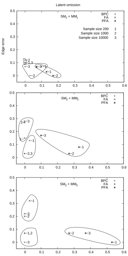
DP3. Discover as many features as possible about the causal relationships among the latents inG.
Since factor analysis addresses only tasks DP1 and DP2, we compare it directly to BuildPureClusterson DP1 and DP2. For DP3, we use our procedure and factor analysis to compute measurement models, then discover as much about the features of the structural model among the latents as possible by applying GES-MIMBuild to the measurement models output by BPC and factor analysis.
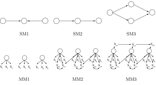
We hypothesized that three features of the problem would affect the performance of the algorithms compared: sample size; the complexity of the structural model; and, the complexity and level of impurity in the generating measurement model. We use three different sample sizes for each study: 200, 1,000, and 10,000. We constructed nine generating latent variable graphs by using all combinations of the three structural models and three measurement models in Figure 6. For structural model SM3, the respective measurement models are augmented accordingly.
MM1 is a pure measurement model with three indicators per latent. MM2 has five indicators per latent, one of which is impure because its error is correlated with another indicator, and another because it measures two latents directly. MM3 involves six indicators per latent, half of which are impure.
SM1 entails one unconditional independence among the latents: L1 is independentL3. SM2 entails one first order conditional independence: L1⊥L3|L2, and SM3 entails one first order conditional independence: L2⊥L3|L1, and one second order conditional independence relation: L1⊥L4|{L2, L3}. Thus the statistical complexity of the structural models increases from SM1 to SM3 and the impurity of measurement models increases from MM1 to MM3.
For each generating latent variable graph, we used the Tetrad IV program3 with the following procedure to draw 10 multivariate normal samples of size 200, 10 at size 1,000, and 10 at size 10,000.
1. Pick coefficients for each edge in the model randomly from the interval [−1.5,−0.5]∪ [0.5,1.5].
2. Pick variances for the exogenous nodes (i.e., latents without parents and error nodes) from the interval [1,3].
3. Available athttp://www.phil.cmu.edu/tetrad.
SM1 SM2 SM3
X1
X9
X8 X7
X6
X5
X4
X2
X3
X1
X9
X8
X7
X6
X5
X4
X2
X3
X X X X
10 11 12 X
13 X
14 15
X16 X X
17 18
X1
X9
X8
X7
X6
X5
X4
X2 X3
X X X X
10 11 12 X
13 X
14 15
MM1 MM2 MM3
Figure 6: The Structural and Measurement models used in our simulation studies.
3. Draw one pseudo-random sample of size N.
We used three algorithms in our studies:
1. BPC: BuildPureClusters+GES-MIMBuild 2. FA: Factor Analysis +GES-MIMBuild
3. P-FA: Factor Analysis + Purify + GES-MIMBuild
BPCis the implementation of BuildPureClustersand GES-MIMBuild described in C. FA involves combining standard factor analysis to find the measurement model withGES-MIMBuild to find the structural model. For standard factor analysis, we used factanalfrom R 1.9 with the oblique rotation promax. FAand variations are still widely used and are perhaps the most popular approach to latent variable modeling (Bartholomew et al., 2002). We choose the number of latents by iteratively increasing its number till we get a significant fit above 0.05, or till we have to stop due to numerical instabilities.
Factor analysis is not directly comparable to BuildPureClusters since it does not generate pure models only. We extend our comparison of BPC and FA by including a version of factor analysis with a post processing step to purify the output of factor analysis.
Purified Factor Analysis, orP-FA, takes the measurement model output by factor analysis and proceeds as follows: 1. for each latent with two children only, remove the child that has the highest number of parents. 2. remove all latents with one child only, unless this latent is the only parent of its child. 3. removes all indicators that load significantly on more than one latent. The measurement model output by P-FA typically contains far fewer latent variables than the measurement model output byFA.
In order to compare the output ofBPC,FA, andP-FAon discovery tasks DP1 (finding the correct number of underlying latents) and DP2 (measuring these latents appropriately),
we must map the latents discovered by each algorithm to the latents in the generating model. That is, we must define a mapping of the latents in the Gout to those in the true graphG. Although one could do this in many ways, for simplicity we used a majority voting rule inBPCandP-FA. If a majority of the indicators of a latentLiout inGout are measures of a latent nodeLj in G, then we map Liout to Lj. Ties were in fact rare, but were broken randomly. At most one latent inGout is mapped to a fixed latentL inG, and if a latent in Gout had no majority, it was not mapped to any latent in G.
The mapping forFAwas done slightly differently. Because the output of FA is typically an extremely impure measurement model with many indicators loading on more than one latent, the simple minded majority method generates too many ties. For FA we do the map- ping not by majority voting of indicators according to their true clusters, but by verifying which true latent corresponds to the highest sum of absolute values of factor loadings for a given output latent. For example, letLout be a latent node inGout. SupposeS1 is the sum of the absolute values of the loadings ofLout on measures of the true latentL1 only, andS2
is the sum of the absolute values of the loadings ofLout on measures of the true latent L2 only. IfS2> S1, we rename Lout asL2. If two output latents are mapped to the same true latent, we label only one of them as the true latent by choosing the one that corresponds to the highest sum of absolute loadings.
We compute the following scores for the output modelGout from each algorithm, where the true graph is labelled GI, and whereG is a purification ofGI:
• latent omission, the number of latents inG that do not appear inGout divided by the total number of true latents inG;
• latent commission, the number of latents in Gout that could not be mapped to a latent in Gdivided by the total number of true latents inG;
• misclustered indicators, the number of observed variables inGout that end up in the wrong cluster divided by the number of observed variables inG;
• indicator omission, the number of observed variables in G that do not appear in theGout divided by the total number of observed variables in G;
• indicator commission, the number of observed nodes in Gout that are not in G divided by the number of nodes in G that are not in GI. These are nodes that introduce impurities in the output model;
To be generous to factor analysis we considered only latents with at least three indicators.
Even with this help, we still found several cases in which latent commission errors were more than 100%. Again, to be conservative, we calculate themisclustered indicators error in the same way as inBuildPureClustersorP-FA. In this calculation, an indicator is not counted as mistakenly clustered if it is a child of the correct latent, even if it is alsoa child of a wrong latent.
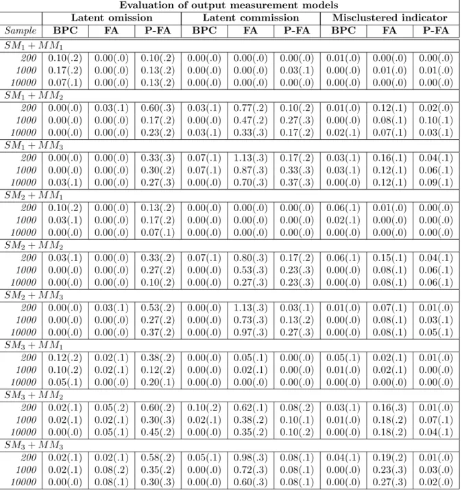
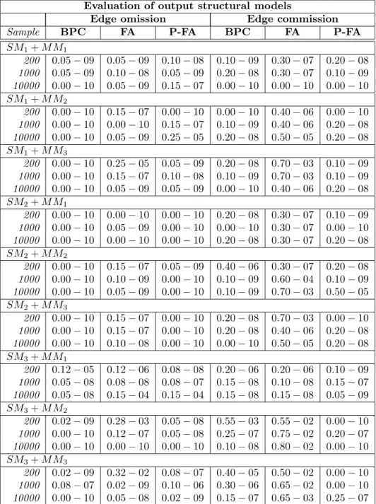
Simulation results are given in Tables 3 and 4, where each number is the average error across 10 trials with standard deviations in parentheses for sample sizes of 200, 1000, 10,000.
Notice there are at most two maximal pure measurement models for each setup (there are two possible choices of which measures to remove from the last latent in MM2 and MM3)
Evaluation of output measurement models
Latent omission Latent commission Misclustered indicator
Sample BPC FA P-FA BPC FA P-FA BPC FA P-FA
SM1+M M1
200 0.10(.2) 0.00(.0) 0.10(.2) 0.00(.0) 0.00(.0) 0.00(.0) 0.01(.0) 0.00(.0) 0.00(.0) 1000 0.17(.2) 0.00(.0) 0.13(.2) 0.00(.0) 0.00(.0) 0.03(.1) 0.00(.0) 0.01(.0) 0.01(.0) 10000 0.07(.1) 0.00(.0) 0.13(.2) 0.00(.0) 0.00(.0) 0.00(.0) 0.00(.0) 0.00(.0) 0.00(.0) SM1+M M2
200 0.00(.0) 0.03(.1) 0.60(.3) 0.03(.1) 0.77(.2) 0.10(.2) 0.01(.0) 0.12(.1) 0.02(.0) 1000 0.00(.0) 0.00(.0) 0.17(.2) 0.00(.0) 0.47(.2) 0.27(.3) 0.00(.0) 0.08(.1) 0.10(.1) 10000 0.00(.0) 0.00(.0) 0.23(.2) 0.03(.1) 0.33(.3) 0.17(.2) 0.02(.1) 0.07(.1) 0.03(.1) SM1+M M3
200 0.00(.0) 0.00(.0) 0.33(.3) 0.07(.1) 1.13(.3) 0.17(.2) 0.03(.1) 0.16(.1) 0.04(.1) 1000 0.00(.0) 0.00(.0) 0.30(.2) 0.07(.1) 0.87(.3) 0.33(.3) 0.03(.1) 0.12(.1) 0.06(.1) 10000 0.03(.1) 0.00(.0) 0.27(.3) 0.00(.0) 0.70(.3) 0.37(.3) 0.00(.0) 0.12(.1) 0.09(.1) SM2+M M1
200 0.10(.2) 0.00(.0) 0.13(.2) 0.00(.0) 0.00(.0) 0.00(.0) 0.06(.1) 0.01(.0) 0.00(.0) 1000 0.03(.1) 0.00(.0) 0.17(.2) 0.00(.0) 0.00(.0) 0.00(.0) 0.02(.1) 0.00(.0) 0.00(.0) 10000 0.00(.0) 0.00(.0) 0.07(.1) 0.00(.0) 0.00(.0) 0.00(.0) 0.00(.0) 0.00(.0) 0.00(.0) SM2+M M2
200 0.03(.1) 0.00(.0) 0.33(.2) 0.07(.1) 0.80(.3) 0.17(.2) 0.06(.1) 0.15(.1) 0.04(.1) 1000 0.00(.0) 0.00(.0) 0.27(.2) 0.00(.0) 0.53(.3) 0.23(.3) 0.00(.0) 0.08(.1) 0.06(.1) 10000 0.00(.0) 0.00(.0) 0.10(.2) 0.00(.0) 0.27(.3) 0.23(.3) 0.00(.0) 0.08(.1) 0.06(.1) SM2+M M3
200 0.00(.0) 0.03(.1) 0.53(.2) 0.00(.0) 1.13(.3) 0.03(.1) 0.01(.0) 0.07(.1) 0.01(.0) 1000 0.00(.0) 0.00(.0) 0.27(.2) 0.00(.0) 0.73(.3) 0.13(.2) 0.00(.0) 0.08(.1) 0.03(.1) 10000 0.00(.0) 0.00(.0) 0.37(.2) 0.00(.0) 0.97(.3) 0.27(.3) 0.00(.0) 0.08(.1) 0.05(.1) SM3+M M1
200 0.12(.2) 0.02(.1) 0.38(.2) 0.00(.0) 0.05(.1) 0.00(.0) 0.05(.1) 0.02(.1) 0.01(.0) 1000 0.10(.2) 0.02(.1) 0.12(.2) 0.00(.0) 0.02(.1) 0.00(.0) 0.01(.0) 0.02(.1) 0.00(.0) 10000 0.05(.1) 0.00(.0) 0.20(.1) 0.00(.0) 0.00(.0) 0.00(.0) 0.00(.0) 0.00(.0) 0.00(.0) SM3+M M2
200 0.02(.1) 0.05(.2) 0.60(.2) 0.10(.2) 0.62(.1) 0.08(.2) 0.03(.1) 0.16(.3) 0.01(.0) 1000 0.02(.1) 0.02(.1) 0.30(.3) 0.02(.1) 0.38(.2) 0.10(.1) 0.01(.0) 0.18(.2) 0.07(.1) 10000 0.00(.0) 0.05(.1) 0.45(.2) 0.00(.0) 0.35(.2) 0.10(.2) 0.00(.0) 0.18(.2) 0.04(.1) SM3+M M3
200 0.02(.1) 0.02(.1) 0.58(.2) 0.05(.1) 0.98(.3) 0.08(.1) 0.04(.1) 0.19(.2) 0.01(.0) 1000 0.02(.1) 0.08(.2) 0.35(.2) 0.00(.0) 0.72(.3) 0.08(.1) 0.00(.0) 0.23(.3) 0.03(.0) 10000 0.00(.0) 0.08(.1) 0.30(.3) 0.00(.0) 0.60(.3) 0.08(.1) 0.00(.0) 0.27(.3) 0.02(.0)
Table 3: Results obtained with BuildPureClusters (BPC), factor analysis (FA) and purified factor analysis (P-FA) for the problem of learning measurement models.
Each number is an average over 10 trials, with the standard deviation over these trials in parenthesis.
and for eachGout we choose our gold standardGas a maximal pure measurement submodel that contains the most number of nodes found inGout.
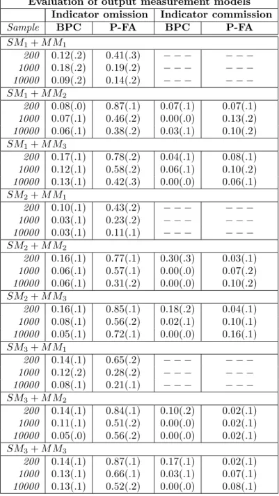
Evaluation of output measurement models Indicator omission Indicator commission
Sample BPC P-FA BPC P-FA
SM1+M M1
200 0.12(.2) 0.41(.3) − − − − − − 1000 0.18(.2) 0.19(.2) − − − − − − 10000 0.09(.2) 0.14(.2) − − − − − − SM1+M M2
200 0.08(.0) 0.87(.1) 0.07(.1) 0.07(.1) 1000 0.07(.1) 0.46(.2) 0.00(.0) 0.13(.2) 10000 0.06(.1) 0.38(.2) 0.03(.1) 0.10(.2) SM1+M M3
200 0.17(.1) 0.78(.2) 0.04(.1) 0.08(.1) 1000 0.12(.1) 0.58(.2) 0.06(.1) 0.10(.2) 10000 0.13(.1) 0.42(.3) 0.00(.0) 0.06(.1) SM2+M M1
200 0.10(.1) 0.43(.2) − − − − − − 1000 0.03(.1) 0.23(.2) − − − − − − 10000 0.03(.1) 0.11(.1) − − − − − − SM2+M M2
200 0.16(.1) 0.77(.1) 0.30(.3) 0.03(.1) 1000 0.06(.1) 0.57(.1) 0.00(.0) 0.07(.2) 10000 0.06(.1) 0.31(.2) 0.00(.0) 0.10(.2) SM2+M M3
200 0.16(.1) 0.85(.1) 0.18(.2) 0.04(.1) 1000 0.08(.1) 0.56(.2) 0.02(.1) 0.10(.1) 10000 0.05(.1) 0.72(.1) 0.00(.0) 0.16(.1) SM3+M M1
200 0.14(.1) 0.65(.2) − − − − − − 1000 0.12(.2) 0.28(.2) − − − − − − 10000 0.08(.1) 0.21(.1) − − − − − − SM3+M M2
200 0.14(.1) 0.84(.1) 0.10(.2) 0.02(.1) 1000 0.11(.1) 0.51(.2) 0.00(.0) 0.02(.1) 10000 0.05(.0) 0.56(.2) 0.00(.0) 0.02(.1) SM3+M M3
200 0.14(.1) 0.87(.1) 0.17(.1) 0.02(.1) 1000 0.13(.1) 0.66(.1) 0.03(.1) 0.07(.1) 10000 0.13(.1) 0.52(.2) 0.00(.0) 0.08(.1)
Table 4: Results obtained with BuildPureClusters(BPC) and purified factor analysis (P-FA) for the problem of learning measurement models. Each number is an average over 10 trials, with standard deviations in parens.
Table 3 evaluates all three procedures on the first two discovery tasks: DP1 and DP2.
As expected, all three procedures had very low error rates in rows involving MM1 and sample sizes of 10,000. Over all conditions, FA has very low rates of latent omission, but very high rates of latent commission, and P-FA, not surprisingly, does the opposite: very