This is known as the standard form of the Van Cittert-Zernike theorem for fixed observers regarding temperature sources [3]. In addition, the analytical derivation of the correlation function gives rise to a relationship linking the measured correlations to the place-dependent brightness temperatures by means of a Highly Oscillatory Integral (HOI) kernel.
Introduction
Le chapitre 3 décrit une première étude du concept d'interférométrie spatio-temporelle combinée à une méthodologie de corrélation temporelle. Une autre étude du concept d'interférométrie spatio-temporelle combinée à une méthodologie de corrélation de fréquence a été détaillée dans le 4ème chapitre.
Publications
Le destin de l'humanité est plus que jamais lié au sort encore incertain de la planète sur laquelle elle évolue. Le réchauffement de l'atmosphère et des océans, l'élévation du niveau des mers et la fonte des glaces aux pôles sont parmi les principaux indicateurs du réchauffement climatique.
Climat terrestre
Une vue d’ensemble
Paramètres déterminants
STATE OF THE ART
AN OVERVIEW OF RECENT MISSIONS
Contents
Introduction
From air campaigns to space missions, microwave remote sensing of the Earth has gained great importance in the scientific community over the decades. The purpose of the present chapter is to provide an overview of L-band dedicated Earth observation missions and techniques using microwave remote sensing.
Introduction to microwave remote sensing
- Why microwave remote sensing ?
- Radiometry
Microwave remote sensing is one of the widespread techniques in Earth observation and is used in particular to monitor key parameters that determine the main exchange processes between the Earth's surface and atmosphere. The large-scale monitoring of Earth's environmental variables is critical to better understanding the interactions at the land/atmosphere interface and provides a valuable foundation for a wide range of scientific applications in hydrology and climatology.
INTRODUCTION TO MICROWAVE REMOTE SENSING
- Active microwave remote sensing
- Passive microwave remote sensing
- Aperture Synthesis
- ESTAR
- SMOS
Aperture synthesis uses the basic idea that the coherent product (cross-correlation) of signals received from a pair of different antennas defines a sample point in the Fourier transform of the luminance temperature map of the observed scene. Then, using inversion and regularization techniques, the illumination temperature distribution of the scene can be reconstructed [9] and the spatial resolution of the reconstructed image is found to be directly dictated by the longer array baseline rather than the antenna diameter in real aperture systems.
![Figure 1.1: Schematic diagram of a two-element interferometer expressed for an ideal two-element interferometer as [8],](https://thumb-eu.123doks.com/thumbv2/1bibliocom/459657.66717/33.918.327.620.97.377/figure-schematic-diagram-element-interferometer-expressed-element-interferometer.webp)
HISTORY OF MICROWAVE REMOTE SENSING
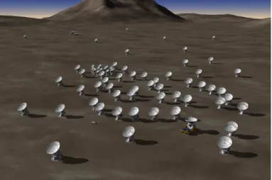
- ALMA
History of microwave remote sensing
- Radars
- Radiometers
Later, the Apollo Lunar Sounder experiment launched in 1972 constituted the first use of a SAR system on board a space instrument. In 1962, radiometric measurements at 15.8- and 22.0-GHz were performed using a two-channel microwave radiometer on board the Mariner 2 spacecraft that provided observations of Venus for the first time [ 14 ].
Rationale for the use of L-Band
Earth observation using microwave remote sensing
- Science motivation
- Soil Moisture (SM)
- Rationale for measuring SM
RETRIEVAL ALGORITHMIC SCHEMES
- How to measure SM ?
- Sea Surface Salinity (SSS)
- Rationale for measuring SSS
- How to measure SSS ?
Retrieval algorithmic schemes
- Iterative approach
- Overview
- Input data
- Iterative retrieval scheme
- Soil moisture retrieval
- Auxiliary inputs
Starting from an initial value of the brightness temperature (TB), the retrieval algorithm aims to iteratively minimize a cost function that takes as its main component the squared weighted differences between the measured and modeled TB for a set of different incidence angles. The iterative minimization of the cost function is performed using the principle of the Levenberg-Marquardt algorithm [22].
RETRIEVAL ALGORITHMIC SCHEMES scattering albedo, surface roughness information, land cover type classification, soil texture, and data
- Tau-omega model
- Soil dielectric models
- Direct model
- Retrieval algorithms
ALGORITHM SCHEMES CONCEAL scattering albedo, surface roughness information, land cover type classification, soil texture and data. The soil moisture acquisition process follows five main steps: .. i) derivation of the emissivity from the observations of TB ase=TB/T with the estimation of the physical surface temperature from the product of the numerical prediction model, . ii) derivation of soil emissivity by eliminating the effects of vegetation, esurf = e−1 +Γ2+ω−ωΓ2.
![Figure 1.8: Contributions to TOA T B [27]](https://thumb-eu.123doks.com/thumbv2/1bibliocom/459657.66717/42.918.297.577.318.571/figure-contributions-to-toa-t-b.webp)
RETRIEVAL ALGORITHMIC SCHEMES 2.5.2 Dual Channel Algorithm (DCA): The Dual Channel Algorithm (DCA) uses both H-
- Sea Surface Salinity retrieval
- Overview
- Algorithm description
1.6.3.2.1 Flat sea: In the case of a smooth surface, the reflectivity is calculated directly through the polarization dependent Fresnel reflection coefficients [37] and is obtained. Therefore, the changes in the local brightness temperature over a large wave (TB,l) relative to TBf lat are a consequence of i) the modification of the angles of incidence and azimuth due to the tilt of the large waves (θl, Φl) and ii) the presence of small-scale diffractive roughness in the large wave.
RETRIEVAL ALGORITHMIC SCHEMES 3.3 Iterative retrieval scheme
- Neural Network approach for SM retrieval
The input vector is multiplied at the level of each neuron of the first layer by a vector of weights and then passed through the corresponding activation function. Again, the output vector of the first layer is subjected to a multiplication by a vector of weights and the resulting linear combination of all is used as input to the neuron of the second layer.
DEDICATED L-BAND EARTH OBSERVATION MISSIONS
Dedicated L-band Earth observation missions
- Soil Moisture and Ocean Salinity (SMOS) mission
- Mission requirements
- SMOS concept
- Use of SMOS data
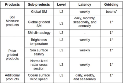
- SMOS products
- Aquarius/SAC-D
- Mission description
- Aquarius instrument
- Use of Aquarius/SAC-D data
- Aquarius/SAC-D products
- Soil Moisture Active and Passive (SMAP) mission
- Introduction
- Mission requirements
- SMAP concept
- Use of SMAP data
- SMAP products
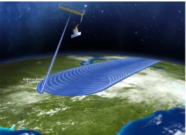
In the field, several reconstruction algorithms based on the Fourier transform relationship between visibilities and TBs and previously described retrieval approaches are launched to reconstruct Earth surface brightness temperature maps. Synchronization between the scatterometer and radiometers allowed simultaneous monitoring of the same ocean pixel in VV, HV, VH, and HH polarization combinations.
![Figure 1.10: SMOS Y-shaped geometry [46]](https://thumb-eu.123doks.com/thumbv2/1bibliocom/459657.66717/48.918.291.594.513.821/figure-smos-y-shaped-geometry.webp)
Summary
PROSPECTS
Prospects
Bibliography
Kerr, “Selecting an optimal configuration for the soil moisture and ocean salinity mission,” Radio Sci., vol. Piepmeier et al., “Radio frequency interference mitigation for the soil moisture active passive microwave radiometer,” IEEE Trans.
EARTH OBSERVATION USERS’ NEEDS
- INTRODUCTION
- Introduction
- Applications
- Study of climate change
- Weather prediction & forecasting
- Drought and flood monitoring
- APPLICATIONS imagery of medium resolution and in-situ measurements so as to detect water level changes and flooded
- Disaster management
- Agriculture and water resources management
- Forest stocks and carbon concentration assessment
- Ocean management
- Challenges
- Users’ needs
- Conclusion
- CONCLUSION knowledge and competences sharing in order to allow a wider exploitation of Earth observation products
Second, the scientific knowledge of various measurement processes and various unwanted interferences needs to be further advanced in order to allow an efficient utilization of Earth observation data. That said, numerous technical and organizational challenges face the development of the new generation of Earth observation missions.
![Figure 2.1: Evolution of US Earth observation dedicated missions [1]](https://thumb-eu.123doks.com/thumbv2/1bibliocom/459657.66717/69.918.240.716.543.810/figure-evolution-earth-observation-dedicated-missions.webp)
TEMPORAL CORRELATION IMAGING
GENERALIZATION OF THE VAN CITTERT–ZERNIKE THEOREM
List of standard parameters
- INTRODUCTION
- Introduction
- Spatio-temporal interferometry
- GENERALIZATION OF THE VAN CITTERT-ZERNIKE THEOREM
- Generalization of the Van Cittert-Zernike theorem
- Introduction
- Model
- Electric field
- GENERALIZATION OF THE VAN CITTERT-ZERNIKE THEOREM measured in the satellite frame R ′ can be obtained from a Lorentz transformation (LT) that describes
- Fourier transform
- Correlation function
- GENERALIZATION OF THE VAN CITTERT-ZERNIKE THEOREM to the time it takes for the satellite to fly over one pixel (with assumed constant temperature). This
- Discussion
- Conclusion
- Similar concepts
- Very Long Baseline Interferometry (VLBI)
- SIMILAR CONCEPTS rid of these corrupting sidelobes is to interpolate the visibilities to the empty regions of the (u, v)-plane
- Application of the generalized VCZT to VLBI
- Conclusion
The spectrum of the electric field received at the satellite's position corresponds to the Fourier transform of. Therefore, the amplitude of the correlation function is suppressed by a factor ∼ vs/c relative to the standard case of ∆t = 0.
3.4.2 2D Doppler-Radiometer
- Introduction
- Concept
- Discussion
- Conclusion
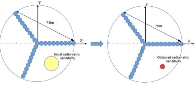
First, to achieve the expected 15 km spatial resolution, the minimum required separation between the antennas is in the order of 50 m. The study of the 2D Doppler radiometer concept showed an expected achievable spatial resolution of the order of 15 km using a 50m-separated three-antenna configuration.
FOURIER CORRELATION IMAGING
ANALYTICAL DERIVATION
Introduction
The basic idea behind spatio-temporal interferometry resulted from the enhanced understanding of the aperture synthesis technique thanks to the SMOS achievements. This is precisely the basis of the spatio-temporal approach that proposes the combination of time-space variables in the correlation procedure.
Theoretical model
- Electric field
Thus, one first wondered whether the generation of virtual longer baselines using the movement of the instrument could have a significant impact on the achieved spatial resolution. A preliminary study of the spatio-temporal interferometry combined with atemporal correlation imaging procedure based on cross-correlation of the temporal samples of the obtained signals at various spatial positions of antennas was carried out in previous chapter.
THEORETICAL MODEL
- Fluctuations of sources
We assume that the current fluctuations of sources on the Earth's surface can presumably be described by Random Gaussian Processes (RGPs).
Fourier Correlation Imaging
- Introduction
FOURIER CORRELATION IMAGING
- Electric field spectrum
- Correlation function
It further shows the coupling between the frequency ω of the electric field spectrum and the frequencies of the source's fluctuations ω′ by means of the Doppler shift. If we denote the frequency response of the entire chain by H(ω), the delivered voltage through the antenna is expressed as follows: ˜Vr(ω) =H(ω) ˜Er(ω).
FOURIER CORRELATION IMAGING the filtered version as follows
Again, if we neglect the weak frequency dependence of the Fourier transform of the current intensities and the weak variation of ω′2 compared to the fast oscillations of the phase factors, which can be extracted from the integral as ω20, the integral over ω′ amounts to 4.25). FOURIER CORRELATION PICTURE where in the phase we neglected the second order termωcβ/c and set K4 = 2πK3ω20.
- Properties of the correlation function
The frequency integral in the previous expression of the correlation function leads to a precise value of the time difference ∆t,. In addition, the motion of the satellite causes the temperature T to depend on the time variable tc as follows: T(r′′+vstc) = T(x′′+x, y′′).
FOURIER CORRELATION IMAGING Equation (4.39) expresses differently the obtained correlation function using the FouCoIm concept com-
- General expression of the correlation function
- Simplified expression of the correlation function
- Study of the HOI kernel
- Approximation of the HOI kernel
On this basis, if we assume that the HOI kernel can be approximated, the reconstruction of the FT from current intensities, and hence brightness temperatures, is thus reduced to a y-direction inversion problem. We further show that (4.46) leads to a 2D representation of the intensity of current fluctuations as a function of position by means of a frequency-dependent (on ωc and ∆ω) integral core function.
- Analytical inversion of the HOI kernel
- Analytical inversion of the correlation function
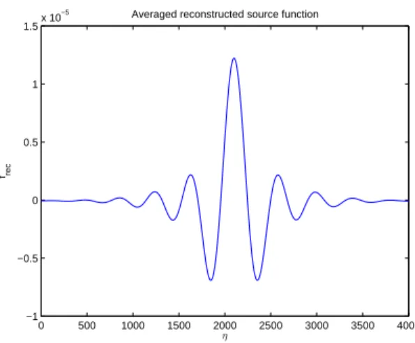
- Reconstructed source function
- Analytical inversion in the case of a single source point
As previously announced, the only relevant regime in the definition of the HOI kernel is β ≫α. We then derive the expression of the correlation function due to a single source with respect to the inversion condition (4.54), equivalent to .
FOURIER CORRELATION IMAGING One finally gets by introducing the filter function
- Estimation of the geometric resolution
- Discussion
Therefore, the best achievable value of the geometric solution in the cross track direction is derived, Rymin(ηs)≡∆rπ(ηs2+θ2)3/2. A first theoretical derivation of the radiometric sensitivity in the simple case of a single source point (not presented here) gave unexpected values and did not allow to draw conclusions.
Appendix: Thermal fluctuations and their fundamental lawslaws
APPENDIX: THERMAL FLUCTUATIONS AND THEIR FUNDAMENTAL LAWS of two sources on the Earth's surface, figures 4.10, 4.11 show the average over the set of realizations of.
APPENDIX: THERMAL FLUCTUATIONS AND THEIR FUNDAMENTAL LAWS of two sources at the Earth’s surface, figures 4.10,4.11 show the average over the set of realizations of
NUMERICAL DERIVATION
Introduction
A discussion of the FDT assumption (equation (4.4)), the verification of which is essential for the space implementation of the FouCoIm concept, is presented at the end of the second section. The full development of this chapter will be the subject of a publication currently under preparation at the time of writing [1].
NUMERICAL QUADRATURE OF THE HIGHLY OSCILLATORY INTEGRAL KERNEL
Numerical quadrature of the highly oscillatory integral kernel
- Introduction
- Theoretical model
- Quadrature methods for highly oscillatory integrals
- Introduction
In what follows, we will be interested in the theoretical and numerical quadrature of the following simplified form of the integral kernel. The need for advanced methods in quadrature of HOIs is a result of the failure of most traditional methods as the frequency of oscillations increases.
NUMERICAL QUADRATURE OF THE HIGHLY OSCILLATORY INTEGRAL KERNEL 3.2 Asymptotics
- Numerical quadrature methods
In the case of an ar-order stationary pointξ, the singularity can be removed by subtracting the ar-term Taylor expansion from f[10], . NUMERIC SQUARE OF THE HIGHLY OSCILLATING INTEGRAL KERNEL 5.2.3.3.1 Filon-type methods The originally developed Filon method consisted of dividing the .
NUMERICAL QUADRATURE OF THE HIGHLY OSCILLATORY INTEGRAL KERNEL 3.3.1 Filon-type methods Filon method, as originally developed, consisted in dividing the
- Analytical derivations of the quadrature
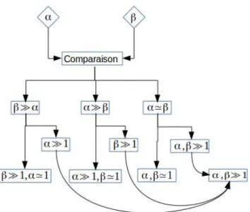
- Frequency regimes
- Analytical derivation of the approximations
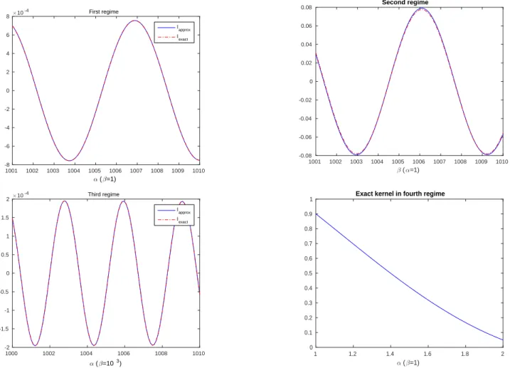
Based on (5.25), the quadrature of the integral kernel in the first regime is performed using a simple trapezoidal rule to calculate I1[f] (due to its non-oscillatory behavior) and a highly oscillatory quadrature method for I2[f]. Furthermore, if we consider the change of variables X =−x, it becomes an integral kernel expression.
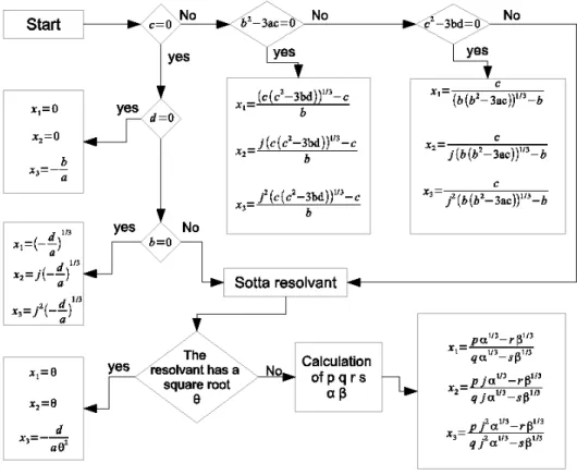
NUMERICAL QUADRATURE OF THE HIGHLY OSCILLATORY INTEGRAL KERNEL In the first regime, an analytical approximation is derived using the stationary phase approxima-
NUMERICAL QUADRATURE OF HIGH OSCILLATORY INTEGRAL KERNEL In the first regime, the analytical approximation is derived using stationary phase approximations. NUMERICAL QUADRATURE OF A HIGHLY OSCILLATORY INTEGRAL KERNEL, which, if we set uv=−p/3, that the following system of Eqs.
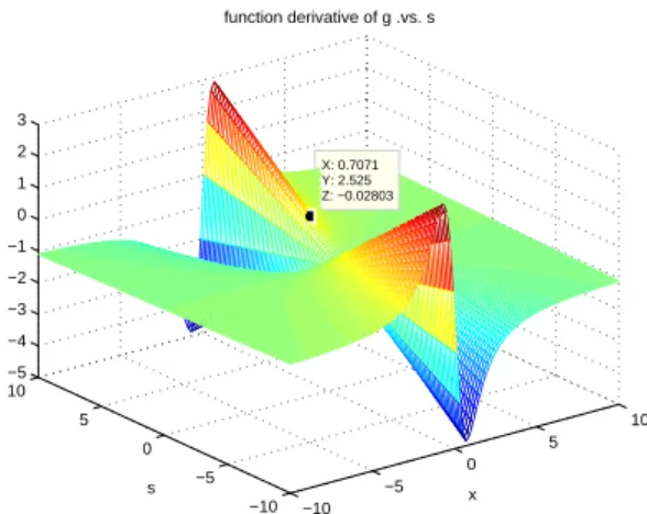
Similar to the direct method, we retain only real non-negative solutions in the determination of the stationary points of function g,. NUMERICAL QUADRATURE OF THE HIGHLY OSCILLATORY INTEGRAL KERNEL5.2.4.2.2 Use of numerical methods: Previous asymptotic approximations of the HOI kernel con-.
NUMERICAL QUADRATURE OF THE HIGHLY OSCILLATORY INTEGRAL KERNEL 4.2.2 Using numerical methods: Previous asymptotic approximations of the HOI kernel con-
As before, in the third regime there is no need to use the numerical method because the integral kernel is not HOI. NUMERICAL SQUARRATION OF A HIGHLY OSCILLATORY INTEGRAL KERNEL Once the ˜F approximation is derived, a Levine-type approximation is then obtained using .
NUMERICAL QUADRATURE OF THE HIGHLY OSCILLATORY INTEGRAL KERNEL Once the approximation ˜F is derived, the Levin-type approximation is afterwards obtained using the
- Quadrature simulation results
- First regime
- Second regime
- Fourth regime
- Discussion
- Conclusions
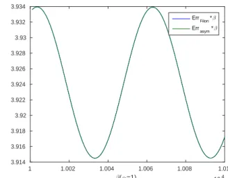
As expected, the Levin- and Filon-type approaches approximate the HOI kernel in the first regime with a quadrature error of the order of O(β-1). The quadrature of the HOI core in the fourth regime (β ≃ α, α, β ≫ 1) is performed by asymptotic (stationary phase approximation and asymptotic expansion) and numerical (Levin-type) methods in the absence and presence of stationary points.
Numerical processor: derivation & results
- Introduction
- Numerical simulations using frequency translation
- Current density
- Correlation function
- Reconstruction procedure using frequency translation
- Simulation results
- Numerical simulations using the quadrature of the HOI kernel
- Introduction
- Correlation function
- Correlation matrix
- Highly oscillatory reconstruction procedure
- Discussion
- Numerical simulations in the ultra-sound regime
- Introduction
- Model
- Direct reconstruction procedure
- Inversion in the case of a single source point
- Reconstructed source function
- Geometric resolution
- Radiometric sensitivity (RS)
- Discussion on the FDT assumption
- Conclusions
This idea originated from the proposal of experimental validation of the FouCoIm concept in the ultrasonic domain. Three different numerical approaches were considered in the numerical study of the FouCoIm concept.
![Figure 1.6: Microwave transmissivity as func- func-tion of increasing biomass [31]](https://thumb-eu.123doks.com/thumbv2/1bibliocom/459657.66717/38.918.526.778.109.414/figure-microwave-transmissivity-func-func-tion-increasing-biomass.webp)
![Figure 1.7: Sensitivity of L-band T B observa- observa-tions as function of soil depth [31]](https://thumb-eu.123doks.com/thumbv2/1bibliocom/459657.66717/38.918.66.375.136.427/figure-sensitivity-band-observa-observa-tions-function-depth.webp)
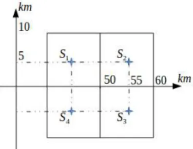
![Figure 1.11: Typical SMOS field of view (X and Y axes are expressed in kilometers) [46]](https://thumb-eu.123doks.com/thumbv2/1bibliocom/459657.66717/49.918.329.639.86.324/figure-typical-smos-field-view-axes-expressed-kilometers.webp)
![Figure 1.13: Aquarius antennas’ beams [55]](https://thumb-eu.123doks.com/thumbv2/1bibliocom/459657.66717/52.918.275.593.776.1059/figure-aquarius-antennas-beams.webp)