Formellement, la contrainte temps réel peut être classée en temps réel dur (HRT temps réel dur), temps réel doux (SRT temps réel doux) et temps réel ferme (temps réel ferme). Nous choisissons de concentrer cette thèse sur l'utilisation de la contrainte (m, k)-firme dans les systèmes adaptatifs temps réel.
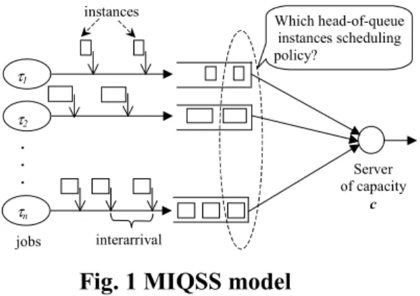
Modèle MIQSS
WFQ et CBQ
Grâce au fait que chaque session possède sa propre file d'attente, seules les sessions mal comportées (envoi de beaucoup de données) sont pénalisées. Parekh [Parekh92] a prouvé que lorsqu'un réseau utilise le GPS et qu'une session est limitée par un bucket qui fuit, la limite de délai de bout en bout peut être garantie.
Modèle de source
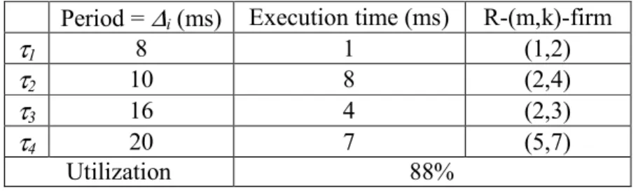
Paramètres des tâches périodiques et sporadiques
Définition traditionnelle
Ce fait nécessite que le processeur ci se voit attribuer des unités de temps pour l'exécution de τi dans l'intervalle [ti,k, ti,k+pi]. Le comportement d'une tâche sporadique τi = (ci, pi) est déterminé par les règles suivantes pour l'instance et l'exécution de τi : Si ti,k est l'heure à laquelle la kième instance de tâche arrive, alors.
Ensemble de tâches concret et abstrait (non concret)
Cette relation s’étend naturellement à une relation entre l’ensemble des tâches concrètes et l’ensemble (non concret) des tâches abstraites. Notez qu'un ensemble de tâches abstraites peut être planifié si et seulement si les tâches peuvent être planifiées pour chaque heure d'activation.
Définition du modèle (m, k)-firm
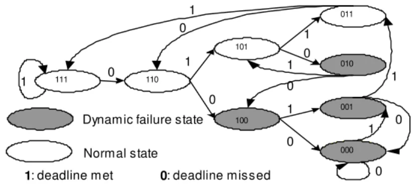
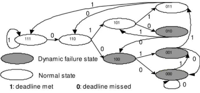
Dans ce qui suit, nous présenterons un système temps réel avec tolérance aux pannes sous la contrainte (m, k)-firm. Une tâche sous contrainte (m, k)-solide peut être dans l'un des deux états suivants : échec normal et échec dynamique [Hamdaoui95].
Ordonnancement sous contraintes « (m, k)-firm »
Ordonnancement avec (m, k) pattern fixe
Dans [Koren95], une condition suffisante est présentée pour déterminer l'ordonnancement d'un ensemble de tâches de « tâches rouges uniquement » avec une priorité attribuée en fonction du « taux monotone », qui est décrit comme suit. Si le motif « Deep Red » (m, k) est planifiable, tous les autres modèles tels que le motif « Sche_mkfirm » et le motif « skip-over » sont également planifiables.
Ordonnancement (m, k) pattern dynamique
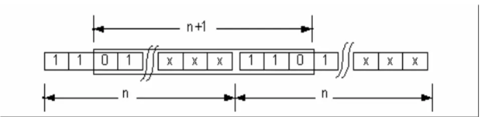
Une séquence k est un mot de k bits, classés du plus récent au plus ancien, dans lequel chaque binaire conserve la mémoire si le délai est manqué (bit = 0) ou respecté (bit = 1), où le bit le plus à gauche représente le plus ancien. Dans la section suivante, la contrainte de fenêtre s'efforce d'améliorer cela en utilisant un quotient de tolérance.
Contrainte de fenêtre « Window constraint »
Comparaison entre (m, k)-firm et contrainte de fenêtre
Comme indiqué précédemment, la contrainte de fenêtre exige qu’il n’y ait pas plus de xi délais manqués dans une fenêtre fixe avec yi dans τi. Bien que la contrainte de fenêtre et la contrainte fixe (m, k) soient mutuellement transformables, elles sont significativement différentes.
Ordonnancement dynamique « Window-contrainte »
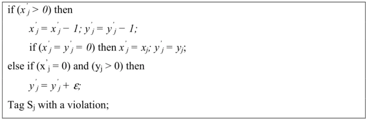
Chaque fois qu'un paquet est transmis dans le flux τi, alors la tolérance de perte de τi est ajustée. La tolérance de perte actuelle est notée x'i/y'i pour tous les paquets alignés fluxτi.
Conclusion
En fait, dans [West99], il est également identifié par l'auteur comme DWCS-2 appelé planification dure utilisant DWCS. Dans le chapitre suivant, nous examinerons les algorithmes de planification dynamique pour obtenir une utilisation plus élevée des ressources.
Condition suffisante d’ordonnançabilité sous NP-DBP-EDF
Motivation de NP-DBP-EDF
Dans ce chapitre, nous considérons uniquement l’algorithme d’ordonnancement dynamique DBP pour un ensemble de tâches sous contraintes (m, k)-firmes. De plus, une politique de planification dynamique peut permettre une meilleure utilisation des ressources disponibles en général.
Analyse des causes du faible taux d’utilisation des ressources
Dans ce chapitre, nous proposerons une version assouplie de la contrainte (m, k)-firm, avec laquelle le système temps réel peut atteindre une utilisation plus élevée des ressources. Nous proposerons une condition suffisante pour dimensionner la ressource système pour l’ensemble des tâches pouvant fournir une version à fenêtre fixe de la contrainte R-(m, k)-firm.
Garantir la contrainte R-(m, k) -firm - gestion des files d'attente
Nous établissons une condition suffisante de la configuration DLB qui permet de fournir une garantie déterministe de contrainte R-(m, k) ferme.
Conclusion et travaux futurs
Conclusion générale
Ainsi, nous avons analysé les raisons du faible taux d'utilisation des ressources dans le domaine de la planification en temps réel d'un ensemble de tâches, et nous ne nous sommes pas limités au cas de la contrainte (m, k)-firme. De plus, le problème général de la planification d'un ensemble de tâches en temps réel sous contrainte HRT et (m, k)-firm s'est avéré être NP-difficile au sens fort et l'utilisation des ressources peut être arbitrairement faible [Garey77] [ Georges00] .
Travaux futurs
Pour l’aspect planification en temps réel, nous avons proposé une condition suffisante qui peut garantir de manière déterministe la limite fixe R-(m, k) pour un ensemble de tâches sous planification à priorité fixe [LiETFA06]. Je tiens à remercier mon co-responsable d'étude, Nicolas NAVET, et la responsable scientifique de TRIO, Françoise SIMONOT-LION, qui ont donné et confirmé cette autorisation et m'ont encouragé à poursuivre ma thèse.
OUTLINE
There are different real-time requirements based on the application's level of fault tolerance. Believing that the (m,k)-firm constraint provides a convenient and powerful framework for determining fault tolerance levels, we decided to focus this thesis on the use of (m,k)-firm constraints in real-time adaptive systems.
General Introduction
1 System model
MIQSS model
WFQ and CBQ
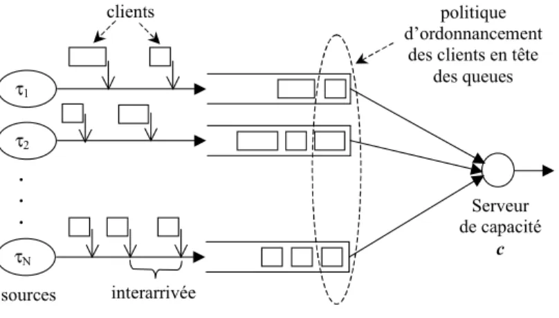
Source model
Periodic and Sporadic: Periodic tasks are real-time tasks that are activated (released) regularly at fixed rates (periods). Sporadic tasks are real-time tasks that fire irregularly at a known bounded rate.
2 Parameters of periodic and sporadic tasks
Traditional definition
The kth execution of taskτi must start no earlier than ti,k and be completed no later than the deadlines of ti,k+pi. The kth execution of taskτi must start no earlier than ti,k and be completed no later than the deadline of ti,k+pi.
Concrete and Abstract Task set
We assume that instances of sporadic tasks are independent in the sense that the time when a sporadic task is called depends only on the time of its last instance and not on the time of any other task instance. Note that the worst-case behavior of a sporadic task τi=(ci, pi) (“worst” in the sense of requiring the most processor time), occurs when τi behaves like a periodic task, that is, τi is called every time pi. steps.
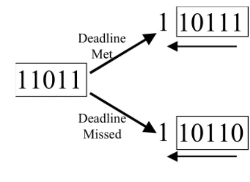
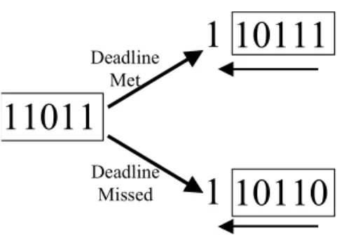
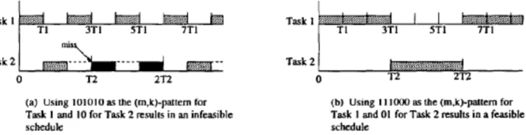
3 (m,k)-firm definition
This diagram describes the state transition of a task, but how to schedule the different tasks is discussed in the next section. To save space and avoid boredom, we will not mention these limitations in the rest of the article.
4 (m,k)-firm scheduling
4.1 (m,k) fixed pattern scheduling
Sche_mkfirm pattern
Note that deep red (m,k) pattern has centralized the WCIP after the release time and can be considered as the worst case of the (m,k) pattern. If Deep Red (m,k) pattern is schedulable, all other patterns like Sche_mkfirm pattern and Skip-over will also be schedulable.
Enhanced Fixed-Priority (m,k)-pattern
However, this deep red (m,k) pattern has low resource usage, and worse, in many cases it requires the same resource to fulfill a (m,k) firm-constrained task set than an HRT-constrained group. task set. This causes the loss of efficiency for the deep red (m,k) pattern, which will be discussed later.
4.2 (m,k) Dynamic scheduling pattern
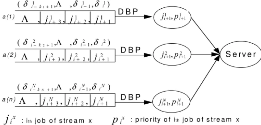
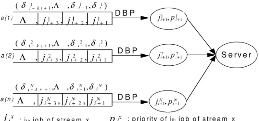
DBP (Distance Based Priority)
In the later part, when the main instances of different tasks have the same priority, EDF (Earliest Deadline First) is used by default. For example, the constraint (2,3)-firm and (3,4)-firm are initially assigned the same priority.
5 Window Constraint
Comparison between (m,k)-firm and window-constraint
In addition, the (m,k)-solid constraint is also proposed for a sliding window that slides period by period. In fact, a sliding window means that the window slides period by period, while a fixed window means that the window slides k-periods by k-periods.
Dynamic Window-constraint Scheduling
- DWCS-1
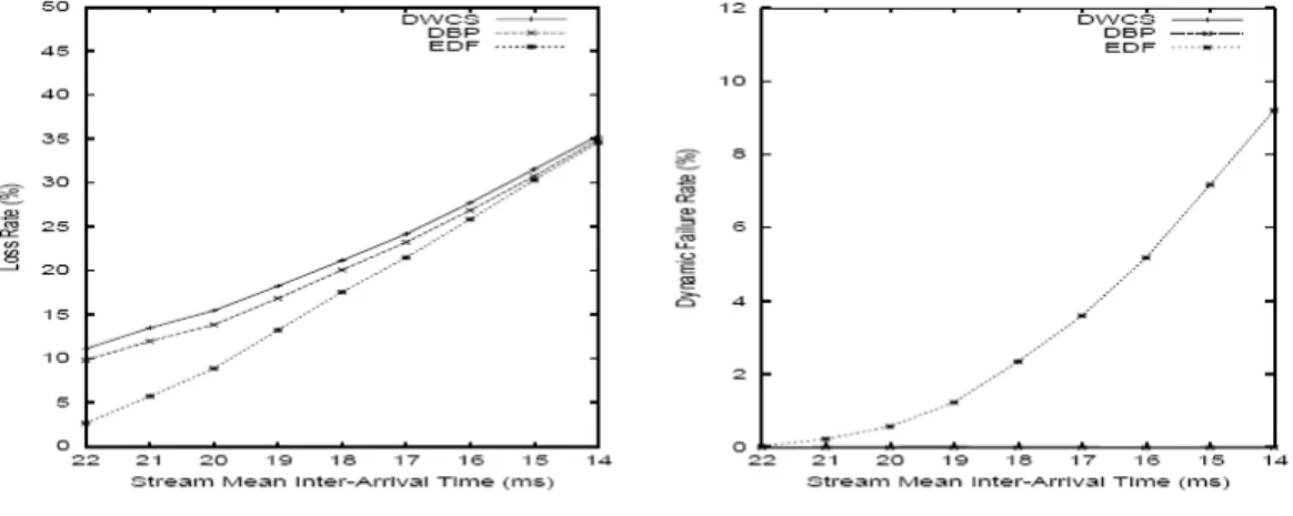
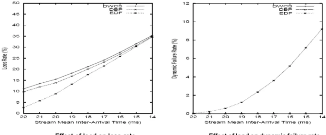
- DBP, DWCS, and EDF Comparisons
- DWCS-2: Hard Real-Time scheduling using DWCS
- Loss-Tolerance Adjustment of DWCS
- Sufficient condition for DWCS-2
- Comments on DWCS-2
Equal terms, sort lowest window constraint first Equal terms and zero window constraint, sort highest window denominator first. In the absence of a feasibility test, window constraint violations are possible.
6 Conclusion
Furthermore, in the next section we will discuss that the proof of the sufficient condition is not correct at all and we will reconstruct it in Appendix A). In the next chapter, we will focus on the dynamic scheduling algorithm to achieve better resource utilization.
NP-DBP-EDF Sufficient Condition
1 Motivation of NP-DBP-EDF
A system is said to be under (m,k)-fixed real-time constraint if it requires guaranteeing the deadline of at least m out of any k consecutive instances of a repetitive task. The priority assignment done online is based on the current state of the system.
2 NP-DBP-EDF scheduling
- NP-DBP-EDF scheduling algorithm
- Busy period and workload evaluation
- NP-DBP-EDF Sufficient Condition theorem
- Sufficient verification length
- Applications of the sufficient condition
- Bandwidth dimensioning for graceful degradation of QoS
- Overload management in automotive control applications
- Discussion on the limits of the deterministic (m,k)-firm guaran- tee
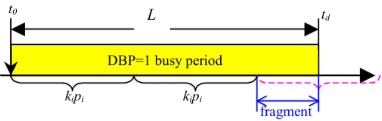
Then, we calculate the narrow upper limit of the workload in the interval L = [tj, td] (see Fig. 14). This is contrary to the fact that in [tj, tj+ci], there is already an executed instance, and there will be only mi-1 DBP=1 instances in [tr-pi,ts-pi].
3 Conclusion
25, we can see that there is an overlap at the initial time. In fact, condition C1 in our theorem can be transformed to be like condition (1) in Jeffay's theorem. Condition C2 in our theorem can also be transformed to be like condition (2) in Jeffay's theorem.
Challenge in Low Utilization Resolution
1 Workload, resource requirement and utilization
Task re-model according to workload
To compare the effectiveness of different scheduling policies, we also consider the utilization of the system resource, which is defined as the ratio between the workload and the resource demand. Note that both the right-hand side of (27) and (28) have been suggested somewhere [West04] [Koubaa04a,b] [Quan00] as using the system.
2 Problem definition
Relation between workload and resource requirement
- Low utilization phenomenon 1
- Low utilization phenomenon 2
- Low utilization phenomenon 3
In the following, we will explain that the resource demand for deterministic guarantees does not depend only on the assigned workload. This indicates that a set of tasks with less load may be more difficult to schedule.
Low utilization theoretical reasons
- Low utilization in HRT
- Low utilization in (m,k)-firm constraint
Since a concrete periodic task set can probably avoid upper critical inter-dispersion, while a sporadic task set (either concrete or non-concrete task set) always suffers from worst-case inter-dispersion. This may therefore explain why a periodic task set has a higher workload but tends to require fewer resources.
Summary of low utilization causes
Then it is natural to find in concrete situations the smaller resource requirement for a task set under given (m,k)-firm or window-constraint, but this problem has been proven NP-hard in a strong sense. The middle vertical line shows that the periodic task set with the highest workload potentially requires less resource, while the sporadic (m,k) firm task set with the least workload potentially requires the most resources.
3 Analysis in Complexity
NP-hard in real-time
- First research direction
- Second research direction
- Third research direction
In general, the general non-occurring periodic task set scheduling under (m,k)-firm constraint has been proved to be a problem of NP-hard in a strong sense [Garey77]. For example, the task set schedulability problem can be solved in polynomial time as long as all tasks are of equal duration as addressed in [Carlier78], [Simons78], [Garey78].
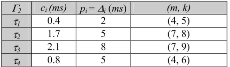
There are still m i jobs that need to be serviced in the next k ipi time units. 34 gives an example of calculating the virtual period (we use the original figure in [Zhang04], where T denotes the period P).
4 Conclusion of perspectives
Consequently, we are motivated to proposed relaxed (m,k)-fixed constraint according to the perspective research methods in the previous chapter. As long as this sufficient condition is satisfied and the instances of each task are selectively abandoned, the QoS of the system can be degraded to the R-(m,k) firm constraint.
1 R-(m,k)-firm scheme
- Definition of R-(m,k)-firm QoS constraint
- R-(m,k)-firm for end-to-end QoS in network
- Demonstration of R-(m,k)-firm advantages by virtual sched- uling pattern
- R-(m,k)-firm is flexible and adaptive
- Limitation of utilization gain for deterministic (m,k)-firm guarantee
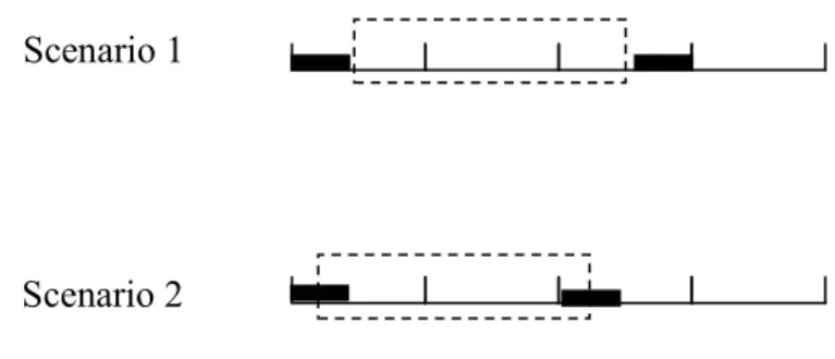
The system must guarantee R-(mi,ki)-firm constraint for each task independently. 4) The real-time constraint includes two factors: (m,k) factor and delay factor. 37 shows the advantage of the R-(m,k)-firm constraint as opposed to the conventional per-packet deadline constraint.
2 Discussing R-(m,k)-firm in MPEG transmission
On the other hand, dropping more instances (or packets) can reduce the delay factor, but risks compromising the (m,k) factor. Therefore, all packages (instances) will be treated equivalently, and the connection between packages at the application level can be ignored.
3 Sufficient condition for R-(m,k)-firm system
Dimensioning method in traditional real-time deadline con- straint
Therefore, we will study the worst case arrival workload to find the resource requirement. In the same way, this method can be extended to calculate the resource requirement for a task set under R-(m,k)-firm constraint.
Periodic characters of Sched_mkfirm pattern
Practically, this method calculates the sum of the workload imposed by higher priority tasks (e.g. in terms of bits) in the interval between the arrival time and the deadline of the instance, as well as the blocking factor of lower priority tasks. Furthermore, from the first instance of the task τi R-(m,k)-hard constraint requires that mi instances must be completed by the end of each ki periods.
Dimensioning for R-(m,k)-firm constraint
Furthermore, the worst interference caused by the higher priority task is the same as in the first case. It is clear that the sum of the total workload in the time interval [ts, td] is smaller than that of Case 1.
4 Simulations to show R-(m,k)-firm advantage in terms of re- source utilization
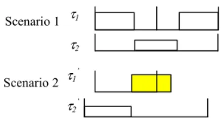
Efficiency of R-(m,k)-firm in admission control
Moreover, in this example, the largest resource demand occurs in the case where an instance of τ1 is blocked by an instance of τ3 due to neglect. Theoretically, the largest resource is still required in the case where an instance of τ1 is blocked by an instance of τ3.
Scheduling trajectory
Therefore, we can show that the resource required by the R-(m,k)-firm constraint is monotonic with respect to workload. This is an expected result, since the R-(m,k)-firm constraint can alleviate the problems in Properties 1 and 2 of Chapter 3.
5 Conclusion
Guarantee R-(m,k)-firm Constraint of Net- work traffic by Queue Management
1 Problem of real-time transmission
2 Queue management introduction
Drop Tail
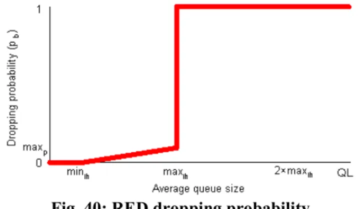
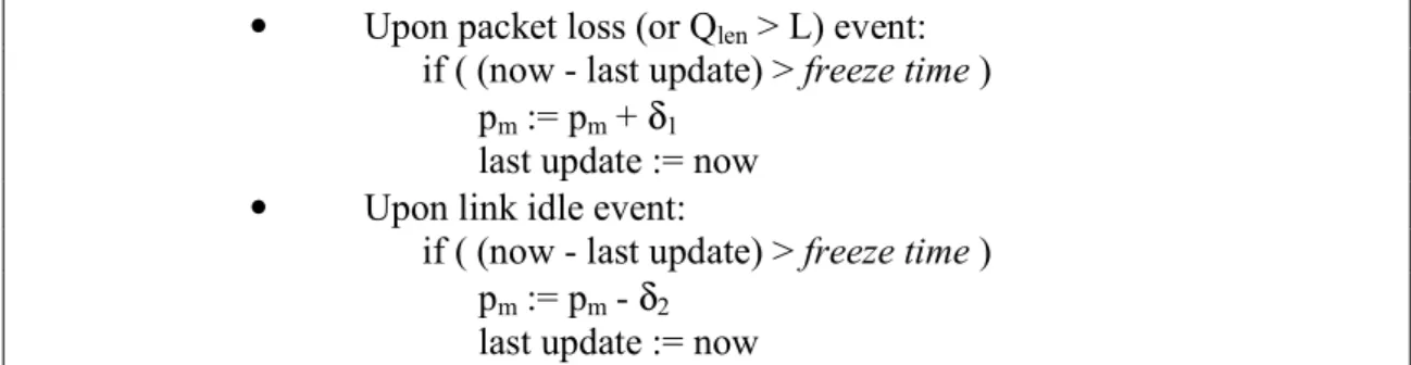
Two thresholds are set to manipulate the dropping process, if the average queue size does not exceed minth, a RED router will not drop any packets, while all arrival packets will be dropped when the average queue size exceeds maxth. Early packet drop starts when the average queue size exceeds minth with the probability given as the following formula and fig.
BLUE mechanism
For connections where extremely large changes in load occur only on the order of minutes, δ1 and δ2 should be set with respect to the freezing time to allow pm to vary from 0 to 1 on the order of minutes. This is in contrast to current queue length approaches where mark and drop probabilities vary from 0 to 1 on the order of milliseconds even under constant load.
Problem of current AQM mechanism for multimedia flows
On typical connections, using freeze time values between 10 ms and 500 ms and setting δ1 and δ2 so that they allow pm to vary from 0 to 1 on the order of 5 to 30 seconds will allow for the BLU control algorithm to work effectively. However, most Internet QoS mechanisms are designed to work with TCP/IP rather than RTP/UDP/IP.
3 R-(m,k)-firm of sliding window constraint
The general definition of the R-(m,k) signature constraint was introduced in the previous chapter, which includes the fixed window version and the sliding window version. Therefore, we will analyze the QoS for the workload in terms of the packet model and the fluid model.
4 DLB (Double-Leaks Bucket)
- Liquid model of DLB mechanism
- Service curve under (r,b)-bounded arrival stream
- Sufficient condition for liquid model of DLB
- Numeric application of liquid DLB
- Packet model of Double-Leaks Bucket
- Sufficient condition of DLB in packet model
- Numeric application of packet DLB model
The DL control switch operates depending on the amount of workload (represented by the height of the water in the bucket and indicated by q). While increasing the water height, the DLB switch remains closed until the height increases to q2.
5 Performance comparison
Selective drop of DLB
However, DLB and RED outperform Drop Tail in terms of average queue length and average delay. Moreover, DLB performs much better than RED and Drop Tail in terms of maximum and average consecutive loss.
Discussion among RED, BLUE and DLB
Moreover, the performance of DLB, RED and Drop Tail is shown in Table 10 in terms of queue length, queue delay, loss rate, as well as the maximum and average consecutive loss. In addition, for RED and BLUE there may be a long consecutive decline depending on the likely decline.
Implementation of DLB in Diffserv
Above all, DLB performs well in active queuing domain, but its main advantage is that it can provide a guarantee for real-time multimedia transmissions that are neither affected by RED nor BLUE. Using DLB on each microflow can then achieve more efficient bandwidth utilization than using hard real-time scheduling.
![Fig. 50: An example of DiffServ node [Davie02]](https://thumb-eu.123doks.com/thumbv2/1bibliocom/466595.71280/176.892.282.661.152.383/fig-50-an-example-of-diffserv-node-davie02.webp)
6 Comparison between R-(m,k)-firm and other real-time con- straint relaxation strategies
Comparison by simulation
Moreover, this scenario dealt with the periodic task set, which distinguishes it from the numerical applications given in Section 4. The numerical applications given in Section 4 are applications of DLB to the upper bound tasks of (r,b), while periodic task has less burst .
7 Compare R-(m,k)-firm with other relaxed constraint models
As a result, Pinwheel model can also be transformed from the sliding window version of R-(m,k) firm constraint. Obviously, this model can be considered as the fixed window version of R-(m,k)-firm constraint when lag factor ∆i=pi.
8 Conclusion
Similar to the R-(m,k)-firm constraint, Zhang and West [Zhang04] proposed a relaxed window constraint to obtain utilization, a virtual deadline constraint. The scheduling algorithm, virtual deadline scheduling, applies the P-faire scope strategy to adjust the deadline of instances according to the execution time.
Conclusion and Future Work
1 Overall conclusion
According to various past works [West04] [Zhang04] [Quan00], we derived three prospective research methods to improve the resource utilization for a real-time system: (1) a heuristic method for suboptimal result (2) determining the parameters of the task set (3) releasing the real-time limits. From the perspective of real-time scheduling, we proposed a sufficient offline condition to deterministically provide an R-(m,k)-hard constraint for the task set in the fixed-priority scheduling method [LiETFA06].
2 Future work
In the queuing aspect, we proposed an active queuing mechanism to dynamically drop the packets in case of congestion (network congestion), while still deterministically guaranteeing R-(m,k)-fixed constraint to (r,b) upper bound. flow. In addition, this mechanism can be implemented in Diffserv to provide the QoS guarantee for real-time transmissions [LiAINA06].
1 Error Indications
Furthermore, we must state that Lemma 1 was stated in an ambiguous way and is not correct at all. One understanding is that yi is already fixed and in this condition it is clear that a larger value of xi leads to a smaller utilization factor so that more flows can be allocated (increasing n).
2 Re-proof of the DWCS-2 sufficient condition
Under these conditions, one optimal P-fair window constraint current set is scheduled in state of ni 1(yi xi) 1.0. Lemma B: if a stream set satisfies P-fair window constraint, then it has already satisfied window constraint in [West04].
3 Pseudo-code
The distribution is also done according to the lowest window counter-first order according to Table 2 in [West04]. Although we based on the results in relative paper [Mok01], we gave the proof as above.
Appendix B
Fatality of (m,k)-firm constraint
First, note that the special (m,k)-fixed set is configured according to a large multiple of the LCM in the period, so that the value of mi and ki can be very large. A task cannot know the parameters of the other tasks, and in real networks the tasks start and end at any time.