at high temperature. Part I: Experimental setup and source

(1)

Infrared emission spectroscopy of CO

₂

at high temperature. Part I: Experimental setup and source

characterization

S. Deprazâ,b,c,, M. Y. Perrinâ,b,, A. Soufianiâ,b,∗

aCNRS, UPR 288, Laboratoire EM2C, Grande Voie des Vignes, F-92290 Chˆatenay-Malabry, France

bEcole Centrale Paris, Grande Voie des Vignes, F-92290 Chˆ´ atenay-Malabry, France

cONERA, DEFA/MCTM, BP 72, F-92322 Chˆatillon, France

Abstract

An experimental setup is developed to analyze infrared emission of CO2 plasmas at atmospheric pressure and temperatures up to 5000 K. A microwave discharge is used to produce the hot gas mixture and emission is recorded by a Fourier transform spectrometer with a spectral resolution between 0.01 and 0.1 cm⁻¹. The plasma is confined inside quartz or sapphire tubes which perturb the measurements through refraction, reflection, absorption and emission. We present in this part the experimental setup, an analysis of tube effects, and the characterization of the plasma in terms of temperature and molar fraction distributions using CO emission in the overtone vibrational bands ∆v=2. Analysis of the measurements of CO2 emission in the 2.7 µm and 4.3 µm regions, and comparisons with calculations using different spectroscopic databases are given in the companion paper.

Keywords: FTIR emission spectroscopy, microwave plasma source,

∗Corresponding author. Tel.: + 33 1 41 13 10 71, fax: + 33 1 47 02 80 35 Email address: anouar.soufiani@em2c.ecp.fr(A. Soufiani)

(2)

temperature measurement, tube effects, CO2 infrared radiation 1. Introduction

The knowledge of very high temperature absorption and emission spectra of CO2 remains a challenge for radiative transfer in applications such as combustion and planetary atmospheric entry. Simulations for heated CO2- N2 mixtures at equilibrium have shown for instance that the IR emission of the CO2molecule remains predominant at temperatures as high as 4000 K [1].

Several experimental studies have been devoted to this molecule during the last fifty years. We describe in the following high temperature measurements and try to classify them according to the confinement of the absorbing or emitting gas in tight cells, flows inside heated cells or the use of combustion products.

Tight cells enable accurate measurements with well controlled temperature, pressure and mixture composition. The achievable temperatures are however limited to about 1000 K due to the soldering of the optical windows with the cell or the thermal tolerance of O-rings. Low spectral resolution absorption measurements with tight cells and grating spectrometers were undertaken for instance by Levi Di Leon and Taine [2] at temperatures up to 850 K. Diode laser absorption experiments enable very high spectral resolution but only cover limited spectral ranges. Rosenmann et al [3, 4] have performed such measurements in the 4.3 µm region up to 800 K, and Mi- halcea et al [5] investigated the 2 µm region in order to determine the most suitable absorption lines to be used as a diagnostic tool in combustion applications. Andr´e et al [6] have measured CO2 absorption spectra in the range

(3)

3700–3750 cm⁻¹ using high resolution Fourier transform infrared (FTIR) spectroscopy and optical paths of about 2 m up to 700 K. Lower spectral resolution FTIR measurements were performed by Parker et al [7] around 12 µm up to 800 K and by Medvecz et al [8] who measured absorption spectra of CO/CO2/N2 mixtures up to 1250 K in the 4.3µm region. Phillips [9] has also performed FTIR measurements in the 4.3 µm region up to 1000 K with 0.06 cm⁻¹ spectral resolution and has derived band model parameters from the experimental data.

Higher temperatures can be obtained using heated leaky cells inside fur- naces and flowing gas mixtures. This technique enabled absorption measurements with grating spectrometers up to 1500 K in the 2.7 and 4.3 µm regions at different pressures and optical paths [10, 11]. Such absorption cells were also used in Refs. [12, 13] in association with moderate resolution FTIR spectroscopy up to 1273 and 1373 K respectively.

In more recent studies, Modest and Bharadwaj [14] and Bharadwaj and Modest [15] developed a drop tube technique which enabled FTIR measurements at 4 cm⁻¹ spectral resolution up to 1550 K. They studied the 2, 2.7 and 4.3 µm regions and compared their measurements with several spectroscopic data bases and statistical narrow-band data. The temperature gradients close to the tube end had apparently no significant effects.

Experiments through combustion products enable to reach higher temperatures but are also affected by uncertainties resulting from the partial knowledge of temperature and composition distributions, and boundary effects. Different authors have attempted to produce quasi two dimensional flames to reduce boundary layer effects [16, 17].

(4)

Pioneering studies were conducted by Ferriso and Ferriso et al [18, 19] who used a supersonic kerosene-oxygen burner at stoichiometric composition, and a Foelsch-type nozzle to avoid shock waves and to produce a quasi uniform cone at the exit of the divergent. The mixture temperature was measured by the emission/absorption technique and the composition was calculated at chemical equilibrium. Absorption spectra were recorded at 4 cm⁻¹ spectral resolution in the 4.3 µm region for temperatures up to 3000 K. A similar study was conducted by Coppalle and Vervich [20] who measured low spectral resolution absorption spectra of a methane-oxygen flame at temperatures up to 2900 K in the 4.3µm. Diode laser absorption measurements of a C2H4-air flame have been carried out by Webber et al [21] in the 2µm region. Selected spectral lines were used in this last study to measure the temperature and CO, CO2 and H2O molar fractions.

The aim of the present study is to measure emission spectra from gases produced by a microwave discharge which enables to reach temperatures as high as 6000 K. Particular attention is given to CO2 emission in the 2.7 and 4.3 µm regions at temperatures never reached before and at high to medium spectral resolution. The microwave discharge through a CO2 flow at atmospheric pressure produces a mixture close to local thermodynamic equilibrium (LTE) containing mainly CO2, CO, O2, C2 and atomic O species.

The emission of CO in the ground electronic state in the range 3800-4400 cm⁻¹ allows accurate determination of the radial temperature distribution in the hot parts of the plasma. Local CO2 emission coefficients or line of sight integrated emission intensities can thus be determined and compared to predictions from spectroscopic databases to study their validity at elevated

(5)

temperatures. We present in this part the experimental setup (section 2) and analyze the effects of confinement tubes on plasma emission spectra (section 3). The plasma characterization using CO emission is then presented in section 4.

2. Experimental setup

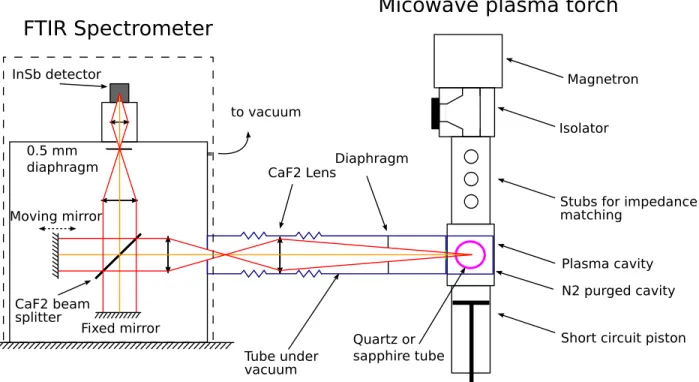
[Figure 1 about here.]

The experimental setup shown on Fig. 1 is aimed at producing and an- alyzing stable plasma flows at high temperature, atmospheric pressure and local thermodynamic equilibrium for different gas mixtures. It is composed of a microwave plasma torch (MPT) which is coupled to an IR Fourier transform spectrometer.

Two different MPT systems were used. The first one (3 kW maximum power) has been originally designed by LITMAS company and the second one (6 kW) by SAIREM company. For both systems, microwaves are gener- ated by a magnetron at 2.45 GHz frequency, pass through an isolator, and then a wave-guide. A triple-head impedance tuner, positioned between the isolator and the plasma cavity, allows to match the impedance in order to decrease the amount of reflected power to less than 1% of the forwarded power.

Adjustment of this tuner is necessary from one experiment to the other as the impedance of the plasma cavity changes with the plasma operating conditions.

The plasma cavity, designed for the purpose of this study, is composed of a WR 340-type aluminum rectangular waveguide, hollowed across its axis to hold a vertical confinement tube of 45 mm outer diameter and 2.5 mm wall

(6)

thickness. The position of the tube within the plasma cavity was calculated so that the electric field of the microwaves is maximum at the center of the tube without plasma. The tangential injection of the gas at the bottom of the cavity produces a swirled gas flow which stabilizes the plasma in the tube center and avoids tube overheating. The plasma produced at atmospheric pressure by this type of devices was analyzed in a previous work using visible and UV emission spectroscopy, and the medium was shown to be very close to thermal and chemical local equilibrium, at least in the central region of the plasma [22, 23]. The first attempt to measure CO2 emission in the 2.7 µm region is also described in Ref. [23] where the optical path was not under vacuum.

The line of sight integrated emission spectra are recorded in the IR range using a high resolution Fourier transform infrared spectrometer (DA8, BOMEM company). The spectrometer is equipped with a CaF2 beam splitter and a liquid nitrogen cooled InSb detector which allow measurements in the near and mid-infrared parts of the spectrum (above 1800 cm⁻¹) at a resolution as high as 4.10⁻³ cm⁻¹. The spectrometer is under vacuum to prevent absorption by CO2 and H2O in ambient air, and the optical path between the MPT and the spectrometer is also under vacuum as shown in Fig. 1. A nitrogen purged cavity is placed around the confinement tube in order to avoid residual absorption outside the tube. This last cavity is made of a refractory material which can operate at high temperature and do not perturb microwave propagation. The spectrometer optical axis is at a height h above the exit of the waveguide; studying the plasma at different horizontal sections defined by the heighthallows us to explore different tem-

(7)

perature profiles and temperature levels since the plasma is cooled down by heat transfer phenomena as hincreases.

The emission spectra are calibrated using the emission of a blackbody radiation source (Landcal company R1200P) at about 900 K with ± 3 K uncertainty. The spatial resolution in the radial direction is determined by the diameter of the pinhole placed in front of the InSb detector (0.5 mm) and from the CaF2 collection lens magnification factor (0.25). This leads to a spatial resolution of about 2 mm. The emission spectra are recorded at different radial positions by moving the microwave plasma torch with a step of 0.5 mm.

The procedure to extract local emission coefficients from line of sight integrated emission intensities, when the medium can be assumed to be optically thin, is based on the classical Abel inversion. The axisymmetry of the calibrated spectra has been checked and a spatial Butterworth-based filter is applied to the intensity curves for each wavenumber. Details on data processing are given in Appendix A. This leads to local absolute emission coefficients (in W.m⁻³.sr⁻¹.(cm⁻¹)⁻¹) in the optically thin regions.

3. Refraction, reflection, absorption and emission by the tube

Plasma confinement inside a quartz or sapphire tube is necessary for the stability of the flow and to avoid diffusion and convection mixing with the outer gaseous medium. However, the tube affects direct measurement of the intensity emitted by the plasma through refraction, reflection, absorption and emission phenomena. The measured temperature on the external wall of the tube reaches 800 K and its own emission is not negligible. The aim of this

(8)

section is to analyze these effects and to determine an accurate procedure for measurement correction when possible. We assume in the following that the plasma and the tube are perfectly axisymmetric and that tube interfaces are smooth so that refraction and reflection can be described by Fresnel’s equations. The tube has an internal diameter R1=20 mm and an external one R2=22.5 mm.

3.1. Refraction effects

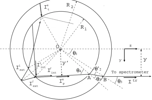
We denote byythe distance between the optical axis of the spectrometer and the line parallel to this axis and crossing the tube center (see Fig. 2), and by y^′ the distance between the tube axis (point O) and the optical path inside the tube that is conjugated with the spectrometer axis through the tube.

Elementary geometrical calculations, using Fresnel’s equations, are re- ported in Appendix B and lead simply to y^′ = y. This important result shows that refraction by quartz or sapphire tubes leads to a deviation of the optical axis but that the optical path associated to the spectrometer axis is not affected by this phenomenon as long as the system can be considered as axisymmetric. Thus, there is no correction to perform in Abel inversion due to refraction. The tube acts however as a slightly divergent lens but this effect, which could affect the spatial resolution of the measurements is neglected in the following.

(9)

3.2. Tube reflection, absorption and emission effects 3.2.1. Optical properties of quartz and sapphire

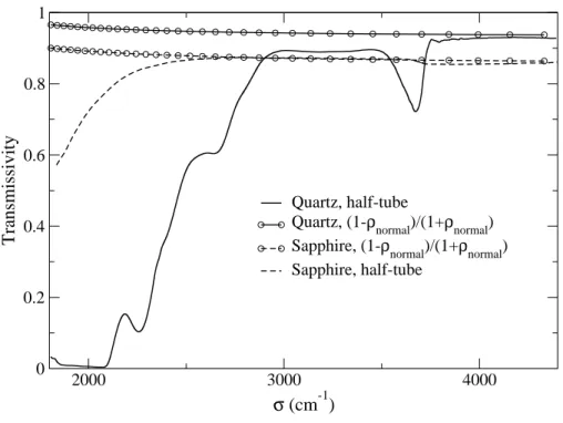
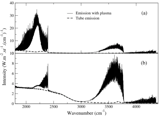
We have measured the transmissivity curves of half-tubes made of quartz and sapphire at room temperature, and the emission curves of the tubes in the plasma operating conditions, just after the extinction of the plasma after each experiment. The last measurements were done at 4 cm⁻¹ spectral resolution to enable fast recording of the spectra before a significant decrease of tube temperature. Examples of these measurements are shown on Fig. 3 for transmission and on Fig. 4 for emission. On this last figure, plasma emission is also presented for comparison. Figure 3 shows also the theoretical normal transmittance, accounting for reflection, but not for absorption, as computed from

Tσ = 1−ρσ(θ = 0)

1 +ρσ(θ = 0), and ρσ(θ = 0) =

nσ −1 nσ + 1

²

, (1)

where ρσ(θ = 0) is the interface normal relectivity, and from the values of the real part of the refractive index nσ, calculated from the Sellmeier-type dispersion relation

n²_λ−1 = B1λ² λ²−C1

+ B2λ² λ²−C2

+ B3λ² λ²−C3

, (2)

with the constants given in Table C.1.

Figure 3 shows first a good agreement between theoretical and measured transmittances in the transparency regions of quartz and sapphire. It shows also that absorption by the tubes occurs below 3700 cm⁻¹ for quartz and 2500 cm⁻¹ for sapphire. This is in agreement with the spectra of the absorption index that may be found in Refs. [24] and [25] for instance, and with

(10)

the present tube emission measurements shown on Fig. 4. Thus, the effects of tube reflection, absorption and emission must be taken into account to correct plasma emission measurements.

[Table 1 about here.]

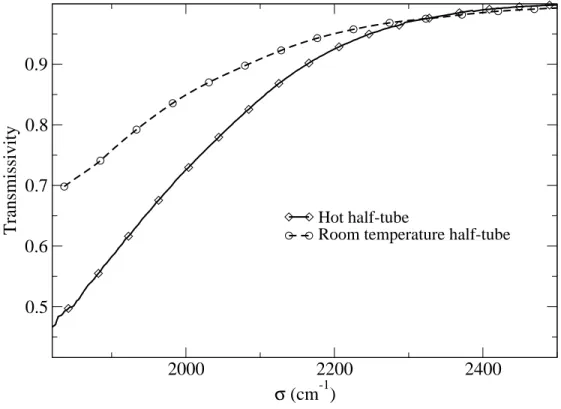
Moreover, it is well known that sapphire absorption coefficient increases with temperature (see e.g. Ref. [25]). We have thus measured the absorption spectrum of the whole sapphire tube just after plasma extinction, using a globar as emission source, and extracted from this measurement, and from the theoretical values of the refractive index, the transmissivity of a half- tube. The result shown on Fig. 5 indicates clearly the strong variation of tube transmissivity with tube temperature. Half-tube transmissivity in the operating conditions will be considered for the analysis of the 4.3 µm CO2

region.

3.2.2. Relation between measured intensity, tube emitted intensity, and plasma emitted intensity

In order to establish the relation between these different intensities, we assume a perfectly axisymmetric geometry, which yields, in association with Fresnel’s equations, remarkable symmetry properties for multiple reflection

(11)

phenomena. Calculation details are given in Appendix C and the general result, accounting for both components of radiation polarization, is

I^tr =a I_pê+b I_tê, (3) where I^tr is the measured intensity, I_pê and I_tê are the intensities emitted by the plasma column and the tube column, and the constantsaandb are given by:

a= τt(1−ρt)(1−ρp)

1−τ_p[ρp+ρ_tτ_t²(1−ρ_p)²], b= (1−ρt) [1−τpρp+τtτp(1−ρp)²] 1−τ_p[ρp+ρ_tτ_t²(1−ρ_p)²] , (4) with the notations given in Appendix C.

Different scenarios can occur depending on the spectral region and the nature of the confinement tube. If the plasma is optically thin (τp ≃1), which is the case for CO2 emission in the 2.7µm region and for CO overtone bands characterized by ∆v=2, and if the tube can be assumed to be transparent (τt≃1,I_t^e≃0, ρ6= 0), Eqs. 3 and 4 reduce to:

I^tr = (1−ρ_t)

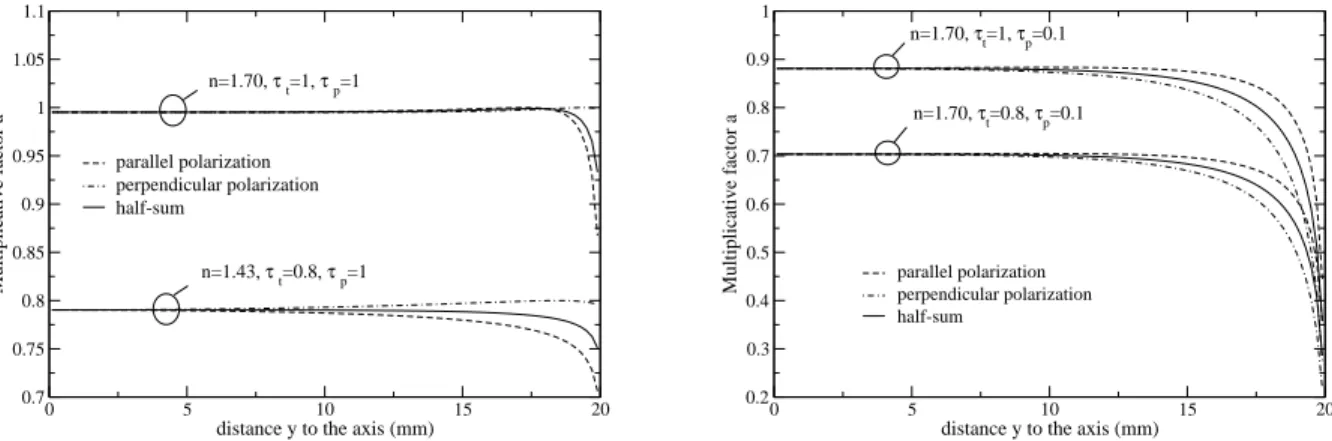
1−ρt(1−ρp)I_p^e. (5) The measured intensityI^tris then equal, to the second order in the reflectivity ρt or ρp, to the intensity emitted by the plasma column. This is easily explained by the fact that the losses by reflection at the tube interfaces are compensated by the intensity emitted by plasma columns symmetrical to the considered column, and reflected by the tube towards the detector. Figure 6 shows that for τp ≃ 1 and τt ≃ 1, the factor a = ¹₂(a_k +a_⊥) remains very close to 1 and the difference is smaller than 0.005 fory <19 mm. This is the reason why the calibration of the intensity with a blackbody source is done without tube.

(12)

For an optically thin plasma (τp ≃ 1) but a partially absorbing tube (τt 6= 1) as for the quartz tube near 3700 cm⁻¹, Figure 6 shows that the factor a is very close to τt (differences limited to 2% for y < 18 mm) and a simple division of the measured intensity by the half-tube transmissivity yields an accurate correction. When the plasma can no longer be considered as optically thin (case of CO2 in the 4.3µm region), reflections by the tube are not compensated by other internal reflections and Fig. 6 shows that, for τp=0.1 for instance, the error introduced by the simple division of I^tr by τt

leads to an underestimation of the plasma intensity by about 13% at y=0.

Measurements of CO2 emission in the 4.3µm region should then be corrected to account for self-absorption. But as the plasma spectral optical thickness is not determined experimentally, this phenomenon will introduce an important source of uncertainty in this spectral region.

Finally, Fig. 4 and Eqs. 3 and 4 show that emission from the tube should be subtracted from the measured intensity to adjust the signal background.

This simple subtraction is rigorous when the plasma is optically thin (τp ≃1) since the measured tube emission is the same with and without plasma, as long as this measurement is carried out very quickly after plasma extinction.

A further correction is required again in the 4.3µm region where the plasma is not optically thin. Figure 4 shows however that sapphire emission remains small in comparison with the maximum level of CO2 emission.

To summarize the above analysis of tube effects, we have shown that refraction effects can be neglected in data processing and put forward the following corrections concerning reflection, emission and absorption:

(13)

• When the plasma is optically relatively thin (2.7 µm region and CO emission in the range 3800< σ <4400 cm⁻¹), reflections of the plasma emitted intensity are compensated by other internal reflections and the intensity calibration must be carried out without tube.

• In the same spectral regions, no further corrections are required for sapphire tubes, while the measured intensity should be divided by the half-tube measured transmissivity τt for quartz tubes.

• tube emission is systematically subtracted from the measured intensity.

The main source of uncertainty due to the confinement tubes results from reflection effects and high plasma optical thickness in the 4.3 µm region.

These phenomena may lead to an underestimation of the measured plasma intensity by about 15%.

4. Source characterization

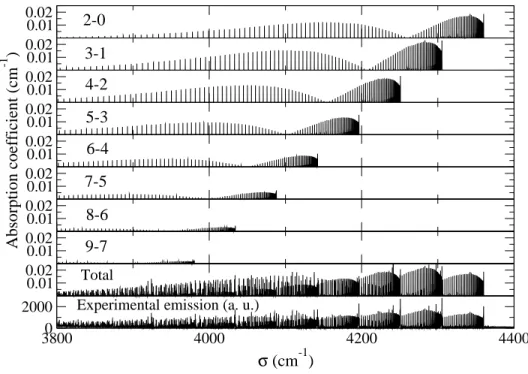
At a given height h above the exit of the microwave cavity, the temperature profile T(r, h) was determined from CO emission in the 4000–4400 cm⁻¹ region. As shown on Fig. 7, CO overtone bands corresponding to

∆v =v^′−v” = 2 are well isolated and the emission signal obviously contains significant contributions from hot bands, up to v^′ =8 or 9, which insures a good sensitivity to the temperature. After calibration and Abel inversion, several techniques can be used to extract the temperature from the local emission spectrum (see e.g. [17]). The Boltzmann method, or the ratio of two selected line intensities is very sensitive to the background continuum, to line overlapping, and to line shapes and broadening parameters. We use

(14)

here a least square adjustment between normalized theoretical spectra and experimental ones to determine the local temperature. In order to avoid the knowledge of CO partial pressure, the measured local emission spectrum, deduced from Abel inversion, is normalized by dividing it by its maximum value, and then compared to normalized theoretical spectra calculated at different temperatures. Comparisons of the absolute levels of the spectra are used afterwards to check the chemical equilibrium hypothesis.

Theoretical line by line calculations of CO spectra, carried out with 0.01 cm⁻¹ spectral resolution, are based on line intensities calculated by Chackerian and Tipping [26] and line positions deduced from the Dunham coefficients given in Ref. [27]. Collisional line broadening coefficients are taken from Ref. [28] for different collision partners. The simple harmonic oscillator (with w=2143.27 cm⁻¹) and rigid rotor model is used for the calculation of the internal partition sum of CO, and is found in very good agreement with direct summation calculations (see e.g. [29, 30]) with differences less than 3%

for temperatures up to 7000 K. We have also checked that line positions and intensities agree well (typically within less than 0.003 cm⁻¹ for positions and 2% for intensities) with the HITRAN data [31] for the cold lines belonging to this last data base, and with HITEMP data [32] with the same accuracy.

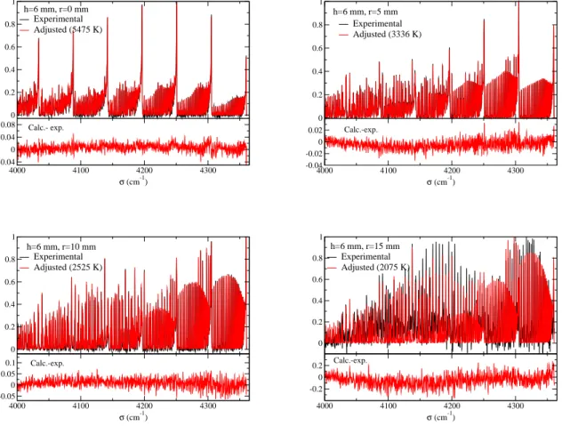
In order to avoid important differences between theoretical and experimental spectra resulting from different line shapes and from FTIR apparatus function, both spectra are convolved with a triangular function of 0.8 cm⁻¹ spectral resolution at the triangle base before the least square adjustment.

(15)

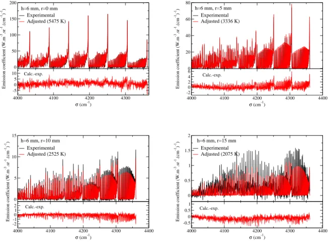
Examples of measured and theoretical CO overtone spectra, calculated at the temperature yielding the least square difference, are shown in Fig. 8 for a height above the plasma cavity h=6 mm and for different radii. The plasma is confined in a quartz tube in this example. The agreement is very good in the central regions with differences limited to a few percents of the maximum signal. At the center of the plasma, the measured temperature is about 5475 K and band heads up to v^′=8 are clearly identified. Higher differences are observed in the outer regions of the plasma where CO emission becomes weak. However, the difference between calculated and measured normalized emission coefficients do not present a spectral structure, corre- lated with the emission coefficient itself, which indicates that the medium is very close to local thermodynamic equilibrium with a single temperature Boltzmann distribution of vibrational and rotational CO levels.

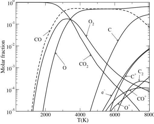
In order to check chemical equilibrium, we compare in the following the absolute levels of the measured and calculated emission coefficients. The latter require however the knowledge of CO molar fraction. Assuming local chemical and thermodynamic equilibrium at the measured temperature, the local composition of the medium is computed by solving the law of mass action for dissociation (Guldberg-Waage equation) and for ionization (Saha equation) reactions, together with electrical neutrality, the perfect gas law and the total conservation of the nuclei [1, 29]. The retained chemical species for CO2 plasmas are CO2, CO, O2, C2, C, O, C⁺, O⁺, CO⁺ and e⁻. Figure 9 shows the computed composition in the temperature range of interest. CO

(16)

molar fraction becomes less than 0.01 for T <1600 K and CO emission is expected to be very low on the periphery of the plasma.

Comparisons between absolute levels of local emission coefficients are given in Fig. 10 for the same experiment as in Fig.8. Here again, a good agreement is observed in the central region of the plasma indicating the reliability of temperature measurement and of chemical equilibrium assumption. For r=10 andr=15 mm, the calculated emission level is smaller than the experimental one with typical differences of about 15% and 30% respectively. As displayed in Fig.9, CO molar fraction is very sensitive to the temperature in the 2000–2500 K range. If we assume chemical equilibrium and use the absolute emission spectrum to adjust the local temperature, we find for instance 2567 K instead of 2525 K for r=10 mm and 2150 K instead of 2075 K for r=15 mm. The spectral structure of the residual in this last adjustment becomes however more pronounced. So, a plausible explanation of the differences observed on the borders of the plasma is a departure from chemical equilibrium. CO concentration is however very small in these regions and does not affect significantly CO2 concentration. Indeed, the experimental CO emission spectrum is about one hundred times smaller atr=15 mm than at the plasma center.

Figure 11 displays typical temperature profiles determined from the normalized and from the absolute CO emission spectra with a confinement tube in

(17)

quartz and at the heighth=6 mm. At this height, the very high temperature narrow central region shown in the figure is confirmed visually by the high luminosity of this region in the visible range. As CO concentration becomes too small on the boundaries (r >15 mm), its emission signal becomes very weak and unusable to determine the temperature. The temperature profile is thus extrapolated in these regions by using the last reliable measurement point using CO spectra and wall temperature. The latter has been measured at the external tube wall by a contact K-type thermocouple and was found in the range 800±50 K for the heights hconsidered here. Two types of extrap- olations where assumed, a simple linear one, and a smooth one preserving the temperature derivative at the last measurement points. These extrapola- tions are also shown on Fig. 11. The uncertainty on the temperature profile, especially in the borders of the plasma, will constitute the most important source of uncertainties in this experimental study and will be accounted for when comparing experimental and theoretical CO2 spectra.

Finally, we have compared the measured CO intensities (in absolute levels and without Abel inversion) to the calculated intensities obtained by solving the radiative transfer equation along a ray at different distances y from the plasma axis. The results are plotted in Fig. 12 using both temperature profiles deduced from normalized and absolute CO emission coefficient. The intensities are plotted on Fig. 12 for the central chord (y=0) and for y=5 and y=10 mm. They are not sensitive to temperature extrapolation since CO concentration vanishes at the periphery. A good agreement is obtained

(18)

between these intensities with, as may be expected, a better agreement for the external chords when the temperature profile deduced from absolute levels of CO emission coefficient is used.

5. Summary

An original setup was developed to measure IR emission spectra of gas mixtures at temperatures up to 6000 K. It includes a microwave discharge in a flowing gas, CO2 in the present study, and a high resolution FTIR spectrometer under vacuum.

The optical effects due to the confinement of the gas mixture inside quartz or sapphire tubes were discussed in detail. The analysis and tube transmittance measurements showed that refraction effects may be neglected and that reflection on smooth tube surfaces and absorption by the tube can be accurately taken into account in the spectral regions where the gas mixture is optically thin. Significant uncertainties remain however when the medium is optically thick like for CO2 in the 4.3 µm region.

For CO2 plasma, the temperature radial distribution was determined from CO emission in the 4000–4400 cm⁻¹ spectral range. A least square adjustment between normalized calculated and Abel inverted experimental emission coefficients yielded accurate determination in the central regions of the mixture. In the same regions, the absolute levels of CO local emission confirmed that the atmospheric plasma is at local chemical and thermodynamic equilibrium. However, due to very low CO concentration in the relatively cold

(19)

outer regions, the temperature profile had to be extrapolated in theses regions. The uncertainties resulting from this extrapolation will be accounted for in the comparisons between theoretical and experimental CO2 emission spectra presented in the companion paper.

Acknowledgments

We acknowledge the French National Research Agency (ANR) for partial financial support through the project Rayhen and the funding from the European Community Seventh Framework Program under grant agreement 242311.

(20)

Appendix A. Data processing and Abel inversion

We briefly describe in this appendix the data processing algorithm that enables to transform line of sight integrated intensities of CO overtone emission to local emission coefficients through Abel inversion. This procedure was first developed in Ref. [33] where more details may be found .

If the plasma can be considered as axisymmetric and optically thin for a given wavenumber σ, the measured intensity Iσ(y) at a distance y from the plasma center is given by:

Iσ(y) = 2 Z Rp

y

Jσ(r) rdr

pr²−y² (A.1)

whereJ_σ(r) is the local emission coefficient (inW.m⁻³.sr⁻¹.(cm⁻¹)⁻¹) at radius randRp is the plasma total radius. The emission coefficient is retrieved by the Abel inversion formula:

Jσ(r) =−1 π

Z Rp

r

dIσ(y) dy

dy

py²−r². (A.2) In practice, measurements are carried out with a spatial step ∆y = 0.5 cm on both sides of the plasma center. The signal is then made symmetrical by finding the local extremum corresponding to the plasma center and by averaging the values at equal distances from this center. A Butterworth filter is then applied to eliminate experimental noise, especially at the plasma borders. The transfer function of this filter is given by:

|H(ω)|²= 1 1 + (_ω^ω

c)²ⁿ, (A.3)

where the cutoff frequency ωc was taken equal to 0.4 and the filter order n was fixed to 2. The axisymmetric and filtered signal was then Abel-inverted

(21)

for each wavenumber using a cubic spline method. A local third order poly- namial is used to extrapolate the signal between each couple of adjacent measurement points using the continuity of the polynomials and of their derivatives. Abel inversion reduces then to the calculations of integrals of the form:

Qk(α, β) = Rβ α

y^k

√y²−α² dy, k ≤2, 0≤α≤β ≤Rp (A.4) These integrals have the analytical expressions:











Q0(α, β) = ln

β α +

q

(^β_α)²−1

Q1(α, β) =p

β²−α²

Q2(α, β) = ^α₂²Q0(α, β) + ^β₂Q1(α, β)

(A.5)

Appendix B. Refraction effects

The different anglesθ1toθ4, involved in the following are defined in Fig. 2.

If we assume that the indices of refraction of the plasma and of the outer medium are equal to 1, and denote by n the refraction index of the tube we have

sinθ3 = y R2

; sinθ^′₂ = sinθ3

n = y

nR2

. (B.1)

The distanceAB between the points of the optical path intersecting the tube interfaces can be deduced from

R²₁ =R₂²+AB²−2R2×AB×cosθ^′₂, (B.2)

(22)

and then the angle θ2 from

R²₂ =R²₁+AB²+ 2R1×AB×cosθ2. (B.3) Finally, the distance y^′ is given by

y^′ R1

=sinθ4 =n sinθ2. (B.4) Using the trigonometric relationsin²θ+cos²θ= 1 for the anglesθ2 etθ^′₂, we find respectively

y^′ nR1

2

+

R²₂−R₁²−AB² 2R1AB

²

= 1, (B.5)

y nR2

² +

R²₂−R²₁+AB² 2R2AB

²

= 1. (B.6)

The combination of these two relations leads to y^′ =y.

Appendix C. Relation between the measured intensity and the intensities emitted by the plasma and by the tube

We adopt the following notations (see also Figure 2) and omit subscripts to indicate parallel and perpendicular polarizations which are understood throughout the following notations and relations:

- I^tr: Intensity transmitted to the detector (measured quantity),

-I_p^e: Intensity emitted by a plasma column at the distance yfrom the center (quantity to be compared to theoretical data),

- I_t^e: Intensity emitted by a tube column. As the tube is relatively optically thin, this intensity is assumed to be the same for tube emission in the inward and outward directions,

(23)

- I_intⁱ : Incident intensity on the internal tube interface, - I_extⁱ : Incident intensity on the external tube interface - I_int^l : Intensity leaving the internal tube interface, - I_ext^l : Intensity leaving the external tube interface,

- ρp : Specular reflectivity at tube interface for radiation propagating from the plasma to the tube,

- ρt : Specular reflectivity at tube interface for radiation propagating from the tube to the outer medium,

- τt : Transmissivity of the tube (not accounting for reflections), - τp : Transmissivity of the plasma column.

The two reflectivitiesρp andρt are calculated, for each polarization, from the general expressions related to radiation travelling from mediumiwith real refractive index ni to mediumt with index nt, and neglecting the imaginary part of the index in comparison with its real part:

ρ_k =

nicosθt−ntcosθi

nicosθt+ntcosθi

2

, ρ_⊥=

nicosθi−nt cosθt

nicosθi+ntcosθt

2

. (C.1) The different angles used in this expression are calculated from the expressions given in Appendix B for each distance y to the plasma axis. The axisymmetry of the problem and Eq. C.1 show that ρp, for instance, is also equal to the specular reflectivity at tube interface for radiation propagating from the tube to the plasma, which is required to express I_int^l .

With these notations, one can write the expressions of each intensity and

(24)

for each polarization:

I^tr = (1−ρt)I_extⁱ (C.2)

I_extⁱ = (1−ρp)τtI_intⁱ +I_t^e (C.3)

I_intⁱ = τpI_int^l +I_p^e (C.4)

I_int^l = (1−ρp)τtI_ext^l + (1−ρp)I_t^e+ρpI_intⁱ (C.5)

I_ext^l = ρtI_extⁱ . (C.6)

Equation C.2 means that the measured intensity I^tr is simply equal to the incident intensity on the outer tube interface multiplied by the interface transmission factor (1−ρt). In Eq. C.3, the incident intensity on the outer tube interfaceI_extⁱ is written as the sum of the incident intensity on the inner tube interface, multiplied by a transmission factor, and the intensity emitted by the tube. Equation C.4 reflects the fact that the incident intensity on the inner tube interface is equal to the intensity leaving the inner interface, multiplied by plasma column transmissivity, plus the intensity emitted by this plasma column. In Eq. C.5, the intensity leaving the inner interface is expressed as the sum of three terms, a directly reflected intensity on this interface, a transmitted intensity coming from tube emission, and the transmitted part of the intensity leaving the outer interface. Finally, since no significant radiation comes from outside, the intensity leaving the outer interface is simply expressed in Eq. C.6 as the reflected part of the incident intensity on the same interface.

The solution of this system leads to the expression of I^tr:

I^tr =a I_p^e+b I_t^e, (C.7)

(25)

with

a= τt(1−ρt)(1−ρp)

1−τp[ρp+ρtτ_t²(1−ρp)²], b= (1−ρt) [1−τpρp+τtτp(1−ρp)²] 1−τp[ρp+ρtτ_t²(1−ρp)²] .

(C.8) I^tr appears then to be a linear combination of the intensities emitted by the plasma and by the confinement tube with the constantsaandbdepending on the different reflectivities and transmissivities. Equations C.7 and C.8 are in fact written for each polarization:

I_k^tr =a_kI_kê_p+b_kI_kê_t, (C.9) I_⊥^tr =a⊥I_⊥ê_p+b⊥I_⊥ê_t, (C.10) where the coefficients ak, bk, a⊥ and b⊥ are calculated from Eqs. C.8 with reflectivities ρp andρt depending on the polarization state according to Eqs.

C.1. As the emission by the plasma and the tube are not polarized (I_kê_p = I_⊥ê_p = ¹₂I_pê and I_kê_t=I_⊥ê_t = ¹₂I_tê), the total transmitted intensity is given by:

I^tr =I_k^tr+I_⊥^tr = 1

2(ak+a⊥)I_p^e+ 1

2(bk+b⊥)I_t^e. (C.11)

(26)

References

[1] Babou Y, Rivi`ere Ph, Perrin MY, Soufiani A. Spectroscopic data for the prediction of radiative transfer in CO2-N2 plasmas. JQSRT 2009;110:89 – 108.

[2] Levi Di Leon R, Taine J. Infrared absorption by gas mixtures in the 300-850 K temperature range I–4.3µm and 2.7µm CO2 spectra. JQSRT 1986;35:337 –43.

[3] Rosenmann L, Langlois S, Delaye C, Taine J. Diode-laser measurements of CO2 line intensities at high temperature in the 4.3µm region. J Mol Spec 1991;149:167 –84.

[4] Rosenmann L, Langlois S, Taine J. Diode laser measurements of CO2

hot band line intensities at high temperature near 4.3 µm. J Mol Spec 1993;158:263 –9.

[5] Mihalcea RM, Baer DS, Hanson RK. Diode-laser absorption measurements of CO2 near 2.0 µm at elevated temperatures. Appl Optics 1998;37:8341 –7.

[6] Andr´e F, Perrin MY, Taine J. FTIR measurements of ¹²C¹⁶O2 line positions and intensities at high temperature in the 3700-3750 cm⁻¹ spectral region. J Mol Spec 2004;228:187 – 205.

[7] Parker RA, Esplin MP, Wattson RB, Hoke ML, Rothman LS, Blumberg WAM. High temperature absorption measurements and modeling of CO2 for the 12 micron window region. JQSRT 1992;48:591 –7.

(27)

[8] Medvecz PJ, Nichols KM. Experimental determination of line strengths for selected carbon-monoxide and carbon-dioxyde absorption lines at temperatures between 295 and 1250 K. Appl Spectrosc 1994;48:1442 –50.

[9] Phillips WJ. Band-model parameters for 4.3 µm CO2 band in the 300- 1000 K temperature region. JQSRT 1992;48:91 – 104.

[10] Burch DE, Gryvnak DA. Infrared radiation emitted by hot gases and its transmission through synthetic atmospheres, rept. no. v-1929. Tech.

Rep.; Ford Motor Co., Aeronutronic Div.; 1963.

[11] Darell E, Burch DE, Gryvnak DA. Laboratory investigation of the absorption and emission of infrared radiation. JQSRT 1966;6:229 –40.

[12] Clausen S, Bak J. FTIR transmission emission spectroscopy of gases at high temperatures: Experimental set-up and analytical procedures.

JQSRT 1999;61:131 –41.

[13] Fleckl T, Jager H, Obernberger I. Experimental verification of gas spectra calculated for high temperatures using the HITRAN/HITEMP database. J Phys D-Appl Phys 2002;35:3138 –44.

[14] Modest MF, Bharadwaj SP. Medium resolution transmission measurements of CO2 at high temperature. JQSRT 2002;73:329 –38.

[15] Bharadwaj SP, Modest MF. Medium resolution transmission measurements of CO2 at high temperature-an update. JQSRT 2007;103:146 –55.

(28)

[16] Ludwig CB. Measurements of the curves-of-growth of hot water vapor.

Appl Optics 1971;10:1057 –73.

[17] Soufiani A, Martin JP, Rolon JC, Brenez L. Sensitivity of temperature and concentration measurements in hot gases from FTIR emission spectroscopy. JQSRT 2002;73:317 –27.

[18] Ferriso CC. High temperature spectral absorption of 4.3-micron CO2

band. J Chem Phys 1962;37:1955 –61.

[19] Ferriso CC, Ludwig CB, Acton L. Spectral emissivity measurements of 4.3 µm CO2 band between 2650 and 3000 degrees K. J Opt Soc Am 1966;56:171 –3.

[20] Coppalle A, Vervisch P. Spectral emissivity of the 4.3-µm CO2 band at high temperature. JQSRT 1985;33:465–73.

[21] Webber ME, Wang J, Sanders ST, Baer DS, Hanson RK. In situ combustion measurements of CO, CO2, H2O and temperature using diode laser absorption sensors. Proc Combust Inst 2000;28:407 –13.

[22] Babou Y, Rivi`ere Ph, Perrin MY, Soufiani A. Spectroscopic study of microwave plasmas of CO2 and CO2-N2 mixtures at atmospheric pressure.

Plasma Sources Sci Technol 2008;17(045010).

[23] Depraz S, Soufiani A, Perrin MY, Babou Y. An experimental setup for IR gas radiative property measurements at temperatures up to 6000 K: application to CO2 and CO2-N2 mixtures. In: Proceedings of the ASME 2009 Heat Transfer Summer Conference, HT2009 - paper 88456.

San Francisco; 2009,.

(29)

[24] Dombrovsky L, Randrianalisoa J, Baillis D, Pilon L. Use of Mie theory to analyze experimental data to identify infrared properties of fused quartz containing bubbles. Appl Optics 2005;44:7021 –31.

[25] Thomas ME, Joseph RI, Tropf WJ. Infrared transmission properties of sapphire, spinel, yttria, and AlON as a function of temperature and frequency. Appl Optics 1988;27:239 –45.

[26] Chackerian C, Tipping RH. Vibrational-Rotational and Rotational In- tensities for CO Isotopes. J Mol Spec 1983;99:431 –49.

[27] Guelachvili G, De Villeneuve D, Farrenq R, Urban W, Verges J. Dunham coefficients for seven isotopic species of CO. J Mol Spec 1983;98:64 – 79.

[28] Hartmann JM, Rosenmann L, Perrin MY, Taine J. Accurate calculated tabulations of CO line broadening by H2O, N2, O2 and CO2 in the 200- 3000 K temperature range. App Optics 1988;27:3063 –5.

[29] Babou Y, Rivi`ere Ph, Perrin MY, Soufiani A. High-temperature and nonequilibrium partition function and thermodynamic data of diatomic molecules. Int J Thermophysics 2009;30:416 –38.

[30] Capitelli M, Colonna G, Giordano D, Marraffa L, Casavola A, Minelli P, et al. Tables of internal partition functions and thermodynamic properties of high-temperature Mars-atmosphere species from 50K to 50000K. Tech. Rep.; ESA Scientific Technical Review 246; 2005.

[31] Rothman LS, Gordon IE, Barbe A, Chris Benner D, Bernath PF, Birk

(30)

M, et al. The HITRAN 2008 molecular spectroscopic database. JQSRT 2009;110:533 –72.

[32] Rothman LS, Gordon IE, Barber RJ, Dothe H, Gamache RR, Gold- man A, et al. HITEMP, the high-temperature molecular spectroscopic database. JQSRT 2010;111:2139 –50.

[33] Deron C. Rayonnement thermique des plasmas d’air et d’argon : Modélisation des propriétés radiative et étude expérimentale. Thesis, Ecole Centrale Paris, France; 2003.

[34] Malitson IH. Interspecimen comparison of the refractive index of fused silica. J Opt Soc Am 1965;55:1205 –9.

[35] Malitson IH. Refraction and dispersion of synthetic sapphire. J Opt Soc Am 1962;52:1377 –9.

[36] Dombrovsky L, Baillis D. Thermal radiation in disperse systems: An engineering approach. Begell House; 2010.

(31)

List of Figures

1 Experimental setup. . . 33 2 Optical path of a ray aligned with the optical axis of the spec-

trometer and leaving the tube at a distance y from the Oz axis, parallel to the spectrometer axis. . . 34 3 Measured and calculated transmissivities of quartz and sap-

phire half-tubes (2.5 mm width, room temperature). The calculations only take into account reflections at the interfaces while the measurements include also absorption effects. . . 35 4 Calibrated spectra of total emission and emission by the tube

alone ((a) sapphire and (b) quartz) recorded just after plasma extinction at y=0 and h=6 mm. Only the spectral region above 2800 cm⁻¹ is processed for quartz tubes. . . 36 5 Transmissivity (ignoring reflection at the interfaces) of a half-

tube of sapphire (2.5 mm width) at room temperature and in the plasma operating conditions. . . 37 6 Multiplicative factora in the relationI^tr =aI_p^e+bI_t^e for opti-

cally thin (left) and thick (right) plasma. . . 38 7 Calculated absorption coefficient of pure CO at atmospheric

pressure and 3500 K. The 8 first graphs show the contributions of the vibrational bands 2-0 to 9-7 ; the 9th graph shows total absorption spectrum and the 10th graph an example of measured emission spectrum. . . 39 8 Comparison between normalized experimental and adjusted

theoretical CO overtone emission coefficients forh=6 mm and different radii. . . 40 9 Chemical composition (molar fractions) of CO2plasma at equi-

librium and at 1 atm. . . 41 10 Comparison in absolute levels of local emission coefficients of

∆v = 2 CO bands for h=6 mm and different radii. . . 42 11 Temperature profiles deduced from normalized and absolute

CO emission coefficients. quartz confinement tube, h=6 mm, CO2 flow rate = 7.0 l/mn, injected microwave power=1.0 kW. 43

(32)

12 Comparison between absolute levels of chord integrated intensities for the ∆v = 2 CO bands for h=6 mm and different distances to the axis. The temperature profile deduced from normalized CO emission coefficient is used in the left graphs and the one deduced from absolute emission coefficients is used in the right graphs. . . 44

(33)

Magnetron Isolator

Stubs for impedance matching

Plasma cavity

Short circuit piston

Micowave plasma torch

N2 purged cavity

FTIR Spectrometer

Fixed mirror Moving mirror

InSb detector

Tube under vacuum

Quartz or sapphire tube CaF2 beam

splitter

to vacuum

Diaphragm CaF2 Lens

0.5 mm diaphragm

Figure 1: Experimental setup.

(34)

y R

R

2

1

O ^z

y

I^l_ext Iⁱ

ext

I^e_p Iⁱ

intI^l_int I^e_t

I^tr θ²

θ’2

θ¹

θ³ θ⁴

y’

A B

To spectrometer

Figure 2: Optical path of a ray aligned with the optical axis of the spectrometer and leaving the tube at a distancey from theOzaxis, parallel to the spectrometer axis.

(35)

2000 3000 4000 σ (cm^-1)

0 0.2 0.4 0.6 0.8 1

Transmissivity

Quartz, half-tube

Quartz, (1-ρ_normal)/(1+ρ_normal) Sapphire, (1-ρ_normal)/(1+ρ_normal) Sapphire, half-tube

Figure 3: Measured and calculated transmissivities of quartz and sapphire half-tubes (2.5 mm width, room temperature). The calculations only take into account reflections at the interfaces while the measurements include also absorption effects.

(36)

2000 2500 3000 3500 4000 Wavenumber (cm^-1)

0 2 4 6 8 10

Intensity (W.m-2 .sr-1 .(cm-1 )-1 )

Emission with plasma Tube emission

0 10 20 30 40

(a)

(b)

Figure 4: Calibrated spectra of total emission and emission by the tube alone ((a) sapphire and (b) quartz) recorded just after plasma extinction at y=0 and h=6 mm. Only the spectral region above 2800 cm⁻¹ is processed for quartz tubes.

(37)

2000 2200 2400 σ (cm^-1)

0.5 0.6 0.7 0.8 0.9

Transmissivity Hot half-tube

Room temperature half-tube

Figure 5: Transmissivity (ignoring reflection at the interfaces) of a half-tube of sapphire (2.5 mm width) at room temperature and in the plasma operating conditions.

(38)

0 5 10 15 20 distance y to the axis (mm)

0.7 0.75 0.8 0.85 0.9 0.95 1 1.05 1.1

Multiplicative factor a

parallel polarization perpendicular polarization half-sum

n=1.70, τ _t=1, τ _p=1

n=1.43, τ _t=0.8, τ _p=1

0 5 10 15 20

distance y to the axis (mm) 0.2

0.3 0.4 0.5 0.6 0.7 0.8 0.9 1

Multiplicative factor a parallel polarization

perpendicular polarization half-sum

n=1.70, τ_t=1, τ_p=0.1 n=1.70, τ_t=0.8, τ_p=0.1

Figure 6: Multiplicative factor ain the relation I^tr =aI_p^e+bI_t^e for optically thin (left) and thick (right) plasma.

(39)

0.020.01 0.020.01 0.020.01 0.020.01 0.020.01

Absorption coefficient (cm-1 ) 0.020.01 0.020.01 0.020.01 0.020.01

3800 4000 4200 4400

σ (cm^-1) 0

2000

2-0 3-1 4-2 5-3 6-4 7-5 8-6 9-7 Total

Experimental emission (a. u.)

Figure 7: Calculated absorption coefficient of pure CO at atmospheric pressure and 3500 K.

The 8 first graphs show the contributions of the vibrational bands 2-0 to 9-7 ; the 9th graph shows total absorption spectrum and the 10th graph an example of measured emission spectrum.

(40)

0 0.2 0.4 0.6 0.8 1

Experimental Adjusted (5475 K)

4000 4100 4200 4300

σ (cm^-1) -0.04

0 0.04

0.08 Calc.- exp.

h=6 mm, r=0 mm

0 0.2 0.4 0.6 0.8 1

4000 4100 4200 4300

σ (cm^-1) -0.04

-0.02 0

0.02 Calc.-exp.

h=6 mm, r=5 mm

0 0.2 0.4 0.6 0.8 1

4000 4100 4200 4300

σ (cm^-1) -0.05

0 0.05

0.1 Calc.-exp.

h=6 mm, r=10 mm

0 0.2 0.4 0.6 0.8 1

4000 4100 4200 4300

σ (cm^-1) -0.2

0 0.2 Calc.-exp.

h=6 mm, r=15 mm

Figure 8: Comparison between normalized experimental and adjusted theoretical CO overtone emission coefficients forh=6 mm and different radii.

(41)

2000 4000 6000 8000 T(K)

10^-5 10^-4 10^-3 10^-2 10^-1 10⁰

Molar fraction

C CO

O₂

CO₂ O

e^-

O⁺ C⁺

C₂

CO⁺

Figure 9: Chemical composition (molar fractions) of CO₂plasma at equilibrium and at 1 atm.

(42)

0 50 100 150 200

Emission coefficient (W.m-3.sr-1.(cm-1)-1)

4000 4100 4200 4300

σ (cm^-1) -5

0 5

10 Calc.-exp.

h=6 mm, r=0 mm

0 20 40 60 80

4000 4100 4200 4300 4400

σ (cm^-1) -2

0 2 4

6 Calc.-exp.

h=6 mm, r=5 mm

0 5 10 15

Emission coefficient (W.m-3 .sr-1 .(cm-1 )-1 )

4000 4100 4200 4300 4400

σ (cm^-1) -2

-1 0 1

2 Calc.-exp.

h=6 mm, r=10 mm

0 0.5 1 1.5 2

4000 4100 4200 4300 4400

σ (cm^-1) -0.5

0 0.5 1

Calc.-exp.

h=6 mm, r=15 mm

Figure 10: Comparison in absolute levels of local emission coefficients of ∆v= 2 CO bands forh=6 mm and different radii.

(43)

-20 -10 0 10 20 Distance to the center (mm)

1000 2000 3000 4000 5000 6000

Temperature (K)

From normalized CO emission From absolute CO emission Linear extrapolation Smooth extrapolation

Figure 11: Temperature profiles deduced from normalized and absolute CO emission coefficients. quartz confinement tube, h=6 mm, CO₂flow rate = 7.0 l/mn, injected microwave power=1.0 kW.