HAL Id: hal-00530999
https://hal.archives-ouvertes.fr/hal-00530999v1
Preprint submitted on 2 Nov 2010 (v1), last revised 11 Jul 2012 (v5)
HAL is a multi-disciplinary open access archive for the deposit and dissemination of sci- entific research documents, whether they are pub- lished or not. The documents may come from teaching and research institutions in France or abroad, or from public or private research centers.
L’archive ouverte pluridisciplinaire HAL, est destinée au dépôt et à la diffusion de documents scientifiques de niveau recherche, publiés ou non, émanant des établissements d’enseignement et de recherche français ou étrangers, des laboratoires publics ou privés.
Horizontal displacements contribution to tsunami wave energy balance
Denys Dutykh, Dimitrios Mitsotakis, Leonid Chubarov, Yuriy Shokin
To cite this version:
Denys Dutykh, Dimitrios Mitsotakis, Leonid Chubarov, Yuriy Shokin. Horizontal displacements con- tribution to tsunami wave energy balance. 2010. �hal-00530999v1�
WAVE ENERGY BALANCE
DENYS DUTYKH∗, DIMITRIOS MITSOTAKIS, LEONID B. CHUBAROV, AND YURIY I. SHOKIN
Abstract. The main reason for the generation of tsunamis is the deformation of the bottom of the ocean caused by an underwater earthquake. Usually, only the vertical bottom motion is taken into accound while the horizontal displacements are neglected. In the present paper we study both the vertical and the horizontal bottom motion while we propose a novel methodology for reconstructing the bottom coseismic displacements field which is transmitted to the free surface using a new three-dimensional Weakly Nonlinear (WN) approach. We pay a special attention to the evolution of kinetic and potential energies of the resulting wave while the contribution of horizontal displacements into wave energy balance is also quantified. Approaches proposed in this study are illustrated on the July 17, 2006 Java tsunami.
1. Introduction
During the years 2004 to 2006 several interesting tsunami events took place in the Indian Ocean. In December 26, 2004, the Great Sumatra-Andaman earthquake (Mw = 9.1, cf.
C. Ammon et al. (2005), [AJT+05]) generated the devastating Indian Ocean tsunami refered in the literature as the Tsunami Boxing Day 2004 (cf. C. Synolakis & E. Bernard (2006), [SB06]). The local tsunami runups from this event exceeded the height of 34 m at Lhoknga in the western Aceh Province. This and other observations led many researchers to ask whether this tsunami was unusualy large for this specific earthquake size. Later it was shown by E.L. Geist et al. (2006) [GBAT06] that the Great Sumatra-Andaman earthquake is very similar in terms of local tsunami magnitude to past events of the same size, for example appeares similar scales scales with the 1964 Great Alaska earthquake (Mw = 9.2, cf. H. Kanamori (1970) [Kan70]).
On March 28, 2005 another earthquake occured approximately 110 km to the SE from the Great Sumatra-Andaman earthquake’s epicenter. The magnitude of this earthquake was estimated to be Mw = 8.6 ∼8.7 (cf. [LKA+05, Bil05, WIS05]). This event triggered a massive evacuation in the surrounding Indian Ocean countries. However, the March 28, 2005 Northern Sumatra earthquake failed to generate a significant tsunami event. The survey teams reported maximum tsunami runup of 4 m. [GBAT06]. This event can be compared with the 1957 Aleutian earthquake (Mw = 8.6, cf. J.M. Johnson and K. Satake (1993) [JS93]) which produced a maximum tsunami runup of 15 m (see J.F. Lander (1996)
Key words and phrases. tsunami waves; water waves; coseismic displacements; wave energy; finite fault inversion.
∗ Corresponding author.
1
[Lan96]). The deficiency of the March 2005 tsunami is related to the slip concentration in the down-dip part of the rupture zone and to the fact that a substantial part of the vertical displacement occured in shallow waters or on the ground [GBAT06].
By contrast, the smaller July 16, 2006 Java earthquake (Mw = 7.8, cf. C.J. Ammon et al. (2006), [AKLV06]) generated an unexpectedly destructive tsunami wave which affected over 300 km of south Java coastline and killed more than 600 people. Field measurements of runup distributions range uniformely from 5 to 7 m in most inundated areas. However, unexpectably high runup vanues were reported at Nusakambangan Island exceeding the value of 20 m. This tsunami focusing effect could be seemingly ascribed to local site effects.
July 16, 2006 Java tsunami can be compared to a similar event occured on June 2, 1994 at the East Java (Mw = 7.6) (see Y. Tsuji et al. (1995) [TIM+95]). This 1994 Java tsunami produced more than 200 casualties with local runup at Rajekwesi slightly exceeding 13 m.
All these examples of recent and historical tsunami events show that there is a big variaty of local tsunami height and runup with respect to the earthquake magnitude Mw. It is almost obvious that the seismic moment M0 is adequate to estimate far-field tsunami amplitudes. However, tsunami wave energy reflects better the local tsunami severity, while the specific runup distribution depends on bathymetric propagation paths and other site- specific effects. One of the central challenges in the tsunami science is to rapidly assess a local tsunami severity from very first rough earthquake estimations. In the current state of our knowledge false alarms for local tsunamis appear to be unavoidable. The tsunami generation modeling attempts to improve our understanding of tsunami behaviour in the vicinity of the genesis region.
Tsunami generation modeling was initiated in the early sixties by the prominent work of K. Kajiura [Kaj63], who proposed the use of the static vertical sea bed displacement for the initial condition of the free surface elevation. Classically, the celebrated Okada [Oka85, Oka92] and sometimes Mansinha & Smylie1 [MS67, MS71] or Gusiakov [Gus78]
solutions are used to compute the coseismic sea bed displacements. This approach is still widely used by the tsunami wave modeling community. However, some progress has been recently made in this direction [OTM01,DD07c,Dut07, DD09b,RLF+08,SF09,DPD10].
In tsunami wave modeling community the horizontal displacements are often disregarded in the tsunami genesis process. We can quote here a few publications devoted to tsunami waves such as one by D. Stevenson (2005) [Ste05]:
“Although horizontal displacements are often larger, they are unimportant for tsunami generation except to the extent that the sloping ocean floor also forces a vertical displacement of the water column.”
Or another one by G.A. Ichinose et al. (2000) [ISAL00]:
“The initial lake level values were specified by assuming that the lake surface instantaneously conformed to the vertical displacement of the lake bottom while horizontal velocities were set to zero. The effect of horizontal defor- mation on the initial condition is neglected here and left for future work.”
1In fact, Mansinha & Smylie solution is a particular case of the more general Okada solution.
The authors of this article also tended to neglect the horizontal displacements field in pre- vious tsunami generation studies [Dut07,Mit09]. Perhaps, this situation can be ascribed to the work of E. Berg (1970) [Ber70] who showed in the case of the 1964 Alaska’s earthquake (Mw = 9.2) that the input into the potential energy from the horizontal motion is less than 1.5% of that from the vertical movement.
The attitude to horizontal displacements changed after the prominent work by Y. Tan- ioka and K. Satake (1996) [TS96]. According to their computations for the 1994 Java earthquake, the inclusion of horizontal displacements contribution results in 43% increase in maximum initial vertical ground displacement and an increase in the wave amplitudes at the shoreline by 30%. The predicted tsunami runup increases by a factor of two. These striking results incited researchers to reconsider the role of the horizontal sea bed motion.
Hereafter, various tsunami generation techniques which involve only the vertical displace- ment field are referred to as the incomplete scenario. On the contrary, the complete tsunami generation takes also into account the horizontal displacements field.
In the current study we shed some light onto the energy transfer process from an un- derwater earthquake to the implied tsunami wave (in the spirit of the study by D. Dutykh
& F. Dias (2009), [DD09a]), while taking into account and quantifying the horizontal dis- placements contribution into tsunami energy balance. We focus only on the generation stage since the propagation phase and runup techniques are well understood nowadays [Ima96, DKK08, KCY07, DPD10,DKM10].
The present study is organized as follows. In Section 2we present mathematical models used in this study. Specifically, in Sections 2.1 and in Section 2.2 a description of the bottom motion and the fluid layer solution is presented respectively. Some rationale on tsunami wave energy computations is discused in Section 2.2.1. Numerical results are presented in Section 3. Finally, some important conclusions of this study are outlined in Section 4.
2. Mathematical models
Tsunami waves are caused by rapid motion of the seafloor due to an underwater earth- quake over broad areas in comparison to water depth. There are some other mechanisms of tsunami genesis such as underwater landslides, for example. However, in this study we focus on the purely seismic mechanism which occurs most frequently in nature.
Hydrodynamics and seismology are only weakly coupled in the tsunami generation prob- lem. Namely, the released seismic energy is partially transmitted to the ocean through the sea bed deformation while the ocean has obviously no influence onto the rupturing process.
Consequently, our problem is reduced to two relatively distinct questions:
(1) Reconstruct the sea bed deformationh=h(~x, t) caused by the seismic event under consideration
(2) Compute the resulting free surface motion
The way how these questions are answered in our study is explained below in Sections 2.1 and 2.2 respectively.
2.1. Dynamic bottom displacements reconstruction. Traditionally, the free surface initial condition for various tsunami propagation codes (see [TG97, Ima96, IYO06]) is assumed to be identical to the static vertical deformation of the ocean bottom [Kaj70].
This assumption is classically justified by the three following reasons:
(1) Tsunamis are long waves. In this regime the vertical acceleration is neglected with respect to the gravity force
(2) The sea bed deformation is assumed to be instantaneous. It is based on the com- parison of gravity wave speed (200 m/s for water depth of 4 km) and the seismic wave celerity (≈3600 m/s)
(3) The effect of horizontal bottom motion is negligible for tsunami generation since the bathymetry is considered as a perturbation of the flat bottom [Ber70]
We have to say that nonhydrostatic effects as well as finite time source duration have been modeled in several recent studies [TT01, DD07c, FG07, KDD07, DD09b, FM09].
Some attempts have also been made to take into account the horizontal displacements contribution [TS96, GBAT06, SFZ+08].
In the present study we relax all three classical assumptions. The bottom deformation is reconstructed using the finite fault solution as it was suggested in our previous study [DMG10]. However, we extend the previous construction to take into account the horizontal displacements contribution as well. The finite fault solution is based on the multi-fault representation of the rupture [BLM00, JWH02]. The rupture complexity is reconstructed using a joint inversion of the static and seismic data. Fault’s surface is parametrized by multiple segments with variable local slip, rake angle, rise time and rupture velocity. The inversion is performed in an appropriate wavelet transform space. The objective function is a weighted sum of L1, L2 norms and some correlative functions. With this approach seismologists are able to recover rupture slip details [BLM00, JWH02]. This available seismic information is exploited hereafter to compute the sea bed displacements produced by an underwater earthquake with better geophysical resolution.
Let us describe the way of how the sea bed displacements are reconstructed. In this reconstruction procedure we follow the great lines of our previous study [DMG10], while adding new ingredients concerning the horizontal displacements field reconstruction. We illustrate the proposed approach in the case of the July 17, 2006 Java tsunami for which the finite fault solution is available [Ji06].
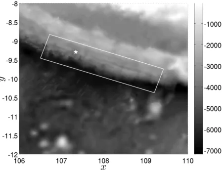
The fault is considered to be the rectangle with vertices located at (109.20508◦ (Lon),
−10.37387◦(Lat), 6.24795km(Depth)), (106.50434◦,−9.45925◦, 6.24795km), (106.72382◦,
−8.82807◦, 19.79951km), (109.42455◦,−9.74269◦, 19.79951km) (see Figure1). The fault’s plane is conventionally divided into Nx = 21 subfaults along strike and Ny = 7 subfaults down the dip angle, leading to the total number ofNx×Ny = 147 equal segments. Param- eters such as subfault location (xc, yc), depthdi, slipui and rake angleφi for each segment can be found at [Ji06] (see also Appendix II, [DMG10]). The elastic constants and pa- rameters such as dip and slip angles which are common to all subfaults are given in Table 1. We underline that the slip angle is measured conventionally in the counter-clockwise direction from the North. The relations between the elastic wave celeritiescp,cs and Lam´e
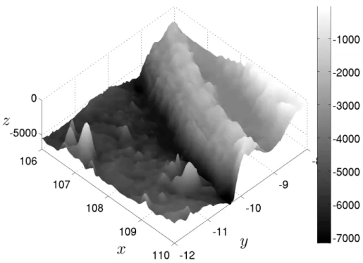
Figure 1. Surface projection of the fault’s plane and the ETOPO1 bathy- metric map of the region we study. The symbol⋆indicates the hypocenter’s location at (107.345◦,−9.295◦). The local Cartesian coordinate system is centered at the point (108◦,−10◦). This region is located between (106◦,−8◦) and (110◦,−12◦).
P-wave celerity cp, m/s 6000 S-wave celerity cs, m/s 3400 Crust density ρ, kg/m3 2700 Dip angle,δ 10.35◦ Slip angle (CW from N) 288.94◦
Table 1. Geophysical parameters used to model elastic properties of the subduction zone in the region of Java.
coefficients λ, µ used in Okada’s solution are classical and can also be found in Appendix III, [DMG10].
One of the main ingredients in our construction is the so-called Okada solution [Oka85, Oka92] which is used in the case of an active fault of small or intermidiate size. The success of this solution may be ascribed to the closed-form analytical expressions which can be effectively used for various modeling purposes involving coseismic deformation.
Remark 1. The celebrated Okada solution[Oka85,Oka92]is based on two main ingredients
— the dislocation theory of Volterra [Vol07] and Mindlin’s fundamental solution for an
elastic half-space [Min36]. Particular cases of this solution were known before Okada’s work, for example the well-known Mansinha & Smylie’s solution [MS67, MS71]. Usually all these particular cases differ by the choice of the dislocation and the Burger’s vector orientation [Pre65]. We recall the basic assumptions behind this solution:
• Fault is immersed into the linear homogeneous and isotropic half-space
• Fault is a Volterra’s type dislocation
• Dislocation has a rectangular shape
For more information on Okada’s solution we refer to [DD07c, DD07a, Dut07].
The trace of the Okada’s solution at the sea bottom (substitutingz = 0 in the geophysical coordinate system) for each subfault will be denoted O(j)i (~x;δ, λ, µ, . . .), where δ is the dip angle, λ, µ are the Lam´e coefficients and dots denote the dependence of the function Oi(j)(~x) on other 8 parameters, cf. [DD07c]. The index i takes values from 1 to Nx ×Ny
and denotes the corresponding subfault segment, while the superscript j is equal to 1 or 2 for the horizontal displacements and to 3 for the vertical component. Hereafter we will adopt the short-hand notation O(j)i (~x) for thejth displacement component of the Okada’s solution for theith segment having in mind its dependence on various parameters.
Taking into account the dynamic characteristics of the rupturing process. We make some further assumptions on the time dependence of displacement fields. The finite fault solution provides us two additional parameters concerning the rupture dynamics — the rupture velocity vr and the rise time tr which are equal to 1.1 km/s and 8 s for July 17, 2006 Java event respectively. The epicenter is located at the point~xe = (107.345◦,−9.295◦) (cf. [Ji06]). Given the origin ~xe, the rupture velocity vr and ith subfault location ~xi, we define the subfault activation times ti needed for the rupture to achieve the corresponding segment i by the formulas:
ti = ||~xe−~xi||
vr
, i= 1, . . . , Nx×Ny.
We will also follow the pioneering idea of J. Hammack [Ham72, Ham73] developed later in [TT01, THT02, DD07c, DDK06, KDD07] where the maximum bottom deformation is achieved during some finite time (known as therise time) according to a specifically chosen dynamic scenario. Various scenarios used in practice (instantaneous, linear, trigonometric, exponential, etc) can be found in [Ham73, DDK06, DD07c]. In this study we adopt the trigonometric scenario which is given by the following formula:
(2.1) T(t) =H(t−tr) + 1
2H(t)H(tr−t) 1−cos(πt/tr) ,
where H(t) is the Heaviside step function. This scenario has an advantage to have also the first derivative continuous at the activation time t = 0. For illustrative purposes this dynamic scenario is represented on Figure 2.
−0.5 0 0.5 1 1.5 2 0
0.1 0.2 0.3 0.4 0.5 0.6 0.7 0.8 0.9 1
t, s
T(t)
Trigonometric scenario
Figure 2. Trigonometric dynamic scenario for tr = 1 s (see J. Hammack (1973), [Ham73]).
We sum up together all ingredients proposed above to reconstruct dynamic displacements field ~u= (u1, u2, u3) at the sea bottom:
uj(~x, t) =
Nx×Ny
X
i=1
T(t−ti)Oi(j)(~x).
Remark 2. We would like to underline here the asymptotic behaviour of the sea bed dis- placements. By definition of the trigonometric scenario (2.1) we have lim
t→+∞T(t) = 1.
Consequently, the sea bed deformation will attain fast its state which consists of the linear superposition of subfaults contributions:
uj(~x, t) =
Nx×Ny
X
i=1
Oi(j)(~x).
Finally, we can predict the sea bed motion by taking into account horizontal and vertical displacements:
(2.2) h(~x, t) = h0(~x+~u1,2(~x, t))−u3(~x, t),
where h0(~x) is a function which interpolates2 the static bathymetry profile given e.g. by the ETOPO1 database (see Figures 1and 4).
Remark 3. In some studies where horizontal displacements were taken into account (cf.
[TS96, BCHK06, SFZ+08, BCD+09]), the first order Taylor expansion was permanently
2In our numerical simulations presented below we use the MATLAB TriScatteredInterp class to interpolate the static bathymetry values given by ETOPO1 database.
applied to the bathymetry representation formula (2.2)to give:
(2.3) h(~x, t)≈h0(~x) +~u1,2(~x, t)· ∇~xh0(~x)−u3(~x, t)
We prefer not to follow this approximation and to use the exact formula (2.2) since it is valid for all slopes (see Figure 4 for Java bathymetry). Another difficulty lies in the estimation of the bathymetry gradient ∇~xh0(x) required by Taylor formula (2.3). The application of any finite differences scheme to the measured h0(~x) leads to an ill-posed problem. Consequently, one needs to apply extensive smoothing procedures to the raw data h0(~x) which induces an additional loss in accuracy.
In the present study we do not completely avoid the computation of the static bathymetry gradient ∇~xh0(~x) since the kinematic bottom boundary condition (2.7) involves the time derivative of the bathymetry function:
∂th =∇~xh0(~x)·∂t~u1,2(~x, t)−∂tu3(~x, t).
The main difference with formula (2.3) is that the former is approximate while the latter is exact.
Another possibility could be to consider static horizontal displacements~u1,2(~x)thus keep- ing dynamics only in the vertical component u3(~x, t). However, we do not choose this option in this work.
In the following section we will present our approach in coupling this dynamic deforma- tion with the hydrodynamic problem to predict waves induced on the Ocean free surface.
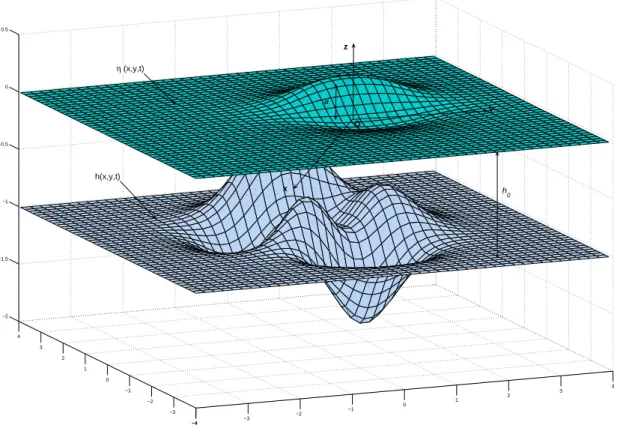
2.2. The water wave problem with moving bottom. We consider the incompressible flow of an ideal fluid with constant density ρ in the domain Ω ⊆ R2. The horizontal independent variables will be denoted by ~x= (x, y) and the vertical one by z. The origin of the Cartesian coordinate system is traditionally chosen such that the surface z = 0 corresponds to the still water level. The fluid domain is bounded below by the bottom z =−h(~x, t) and above by the free surface z = η(~x, t). Usually we assume that the total depth H(~x, t) := h(~x, t) +η(~x, t) remains positive H(~x, t) ≥ h0 > 0 under the system dynamics ∀t ∈[0, T]. The sketch of the physical domain is shown in Figure 3.
Remark 4. Classically in water wave modeling, we make the assumption that the free surface is a graph z = η(~x, t) of a single-valued function. It means in practice that we exclude some interesting phenomena, (e.g. wave breaking phenomena) which are out of the scope of this modeling paradigm.
The governing equations of the classical water wave problem are the following [Lam32, Sto58, Mei94, Whi99]:
∆φ =∇2φ+∂zz2 φ = 0, (~x, z)∈Ω×[−h, η], (2.4)
∂tη+∇φ· ∇η−∂zφ = 0, z =η(~x, t), (2.5)
∂tφ+12|∇φ|2+12(∂zφ)2+gη = 0, z =η(~x, t), (2.6)
∂th+∇φ· ∇h+∂zφ = 0, z =−h(~x, t), (2.7)
−4 −3 −2 −1 0 1 2 3 4
−4
−3
−2
−1 0 1 2 3 4
−2
−1.5
−1
−0.5 0 0.5
z
x
y O
η (x,y,t)
h(x,y,t)
h0 a
Figure 3. Sketch of the physical domain.
with φ the velocity potential, g the acceleration due to gravity force and ∇ = (∂x, ∂y) denotes the gradient operator in horizontal Cartesian coordinates.
Fluid incompressibility and flow irrotationality assumptions lead to the Laplace equation (2.4) for the velocity potential φ(~x, z, t). The main difficulty of the water wave problem lies on the boundary conditions. Equations (2.5) and (2.7) express the free surface and bottom impermeability, while the Bernoulli condition (2.6) expresses the free surface isobarity respectively.
Function h(~x, t) represents the ocean’s bathymetry (depth below the still water level, see Figure3) and is assumed to be known. The dependence on time is included in order to take into account the bottom motion during an underwater earthquake [DD07a, DD07c, DDK06, KDD07, Dut07].
Remark 5. Recently, some weak dissipative effects have also been included into the classical water wave problem (2.4) – (2.7). For more details on the visco-potential formulation we refer to [DDZ08, DD07b,Dut07, Dut09b, Dut09a].
For the exposition below we will need also to compute unitary exterior normals to the fluid domain. It is straightforward to obtain the following expressions for the normals at
the free surface Sf and the bottomSb respectively:
ˆ
nf = 1
p1 +|∇η|2
−∇η
1 , nˆb = 1
p1 +|∇h|2
−∇h
−1 .
In 1968 V. Zakharov proposed a different formulation of the water wave problem based on the trace of the velocity potential at the free surface [Zak68]:
ϕ(~x, t) :=φ(~x, η(~x, t), t).
This variable plays a role of the generalized momentum in the Hamiltonian description of water waves [Zak68, DB06]. The second canonical variable is the free surface elevation η.
Another important ingredient is the normal velocity at the free surface vn which is defined as:
(2.8) vn(~x, t) :=p
1 +|∇η|2 ∂φ
∂nˆf
z=η
= (∂zφ− ∇φ· ∇η)|z=η.
Dynamic boundary conditions (2.5) and (2.6) at the free surface can be rewritten in terms of ϕ, vn and η [CSS92, CS93,FCKG05]:
(2.9) ∂tη− Dη(ϕ) = 0,
∂tϕ+12|∇ϕ|2+gη− 2(1+|∇η|1 2)
Dη(ϕ) +∇ϕ· ∇η2
= 0.
Here we introduced the so-called Dirichlet-to-Neumann operator (D2N) [CM85, CS93]
which maps the velocity potential at the free surface ϕ to the normal velocity vn: Dη : ϕ 7→vn =p
1 +|∇η|2 ∂ˆ∂φn
f
z=η
∇2φ+∂zz2 φ = 0, (~x, z)∈Ω×[−h, η], φ =ϕ, z =η,
p1 +|∇h|2 ∂φ
∂ˆnb
=∂th, z =−h.
The name of this operator comes from the fact that it makes a correspondance between Dirichlet dataϕ and Neumann datap
1 +|∇η|2 ∂φ
∂nˆf
z=η
at the free surface.
So, the water wave problem can be reduced to a system of two PDEs (2.9) governing the evolution of the canonical variablesη andϕ. In order to solve this system of equations we have to be able to compute efficiently the D2N map Dη(ϕ). We will use the Weakly Nonlinear (WN) method described in [DMG10]. It relies on the approximate solution of the 3D Laplace equation in a perturbed strip-like domain using the Fourier transform ( ˆϕ:=F[ϕ],η =F−1[ˆη]):
Dˆη(ϕ) = ˆϕ|~k|tanh(|~k|H) + ˆfsech(|~k|H)− Fh F−1
i~kϕˆ
· F−1 i~kηˆi
, where~k is the wavenumber and f is the bathymetry forcing term
f(~x, t) := −∂th− ∇φ|z=−h· ∇h.
Several details on the time integration procedure can be also found in [DMG10]. Basically, the main idea to integrate exactly in time the linear terms is due to D. Clamond and his collaborators [FCKG05]. The resulting method is only weakly nonlinear and analogous at some point to the first order approximation model proposed in [GN07].
This method was validated in [DMG10] by comparisons with the numerically exact Tanaka solution [Tan86]. Recently it was shown that a tsunami generation process is essentially linear [KDD07,SF09]. Consequently, our WN approach will allow us to observe some nonlinear effects if locally they are important. This is possible when the generation region involves a wide range of depths from deep to shallow regions (see Figures 1and 4).
2.2.1. Tsunami wave energy. In this study we are more particularly interested in the evolu- tion of the generated wave energy [DD09a]. In free surface incompressible flows, the kinetic and potential energies (denoted K and Π correspondingly) are completely determined by the velocity field and the free surface elevation:
K(t) := ρ 2
Zη
−h
Z Z
Ω
|∇φ|2 d~x dz, Π(t) := ρg 2
Z Z
Ω
η2 d~x.
The definition of the kinetic energy K involves an integral over the three dimensional physical domain Ω×[−h, η]. We can reduce the integral dimension using the fact that the velocity potential φ is a harmonic function:
|∇φ|2 =∇ ·(φ∇φ)−φ ∆φ
|{z}
=0
≡ ∇ ·(φ∇φ).
Consequently, the kinetic energy can be rewritten as follows:
K(t) = ρ 2
Z Z
Sf+Sb
∇ ·(φ∇φ)dσ = ρ 2
Z Z
Ω
ϕDη(ϕ)d~x
| {z }
(I)
+ρ 2
Z Z
Ω
φ∂ˇ th d~x
| {z }
(II)
,
where ˇφ denotes the trace of the velocity potential at the bottom φ|z=−h (see D. Clamond
& D. Dutykh (2010), [CD10]). The first integral (I) is classical and represents the change of kinetic energy under the free surface motion while the second one (II) is the forcing term due to the bottom deformation. The total energy3 is defined as the sum of kinetic and potential ones:
E(t) :=K(t) + Π(t) = ρ 2
Z Z
Ω
ϕDη(ϕ)d~x+ ρ 2
Z Z
Ω
φ∂ˇ th d~x+ρg 2
Z Z
Ω
η2 d~x.
Below we will compute the evolution of the kinetic, potential and total energies beneath moving bottom.
3The total energy is normally a conserved quantity but in this study we have an external forcing term (II) coming from the bottom kinematic boundary condition.
Figure 4. Side view of the bathymetry, cf. also Figure 1.
3. Numerical results
The proposed approach will be directly illustrated on the Java 2006 event. The July 17, 2006 Java earthquake involved thrust faulting in the Java’s trench and generated a tsunami wave that inundated the southern coast of Java [AKLV06, FKM+07]. The estimates of the size of the earthquake (cf. [AKLV06]) indicate a seismic moment of 6.7×10²⁰ N · m, which corresponds to the magnitude Mw = 7.8. Later this estimation was refined [Ji06] to Mw = 7.7. Like other events in this region, Java’s event had an unusually low rupture speed of 1.0 – 1.5 km/s (we take the value of 1.1 km/s according to the finite fault solution [Ji06]), and occurred near the up-dip edge of the subduction zone thrust fault. According to C. Ammonet al [AKLV06], most aftershocks involved normal faulting.
The rupture propagated approximately 200 km along the trench with an overall duration of approximately 185 s. The fault’s surface projection along with ocean ETOPO1 bathymetric map are shown on Figures 1 and 4. We note that Indian Ocean’s bathymetry considered in this study varies between 7186 and 20 meters in the shallowest region which may imply local importance of nonlinear effects.
Remark 6. We have to mention that the finite fault inversion for this earthquake was also performed by the Caltech team [OK06]. They estimated the July 17, Southern Java earth- quake magnitude to be Mw = 7.9. In this study we do not present numerical simulations
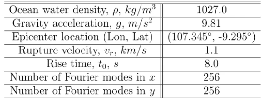
Ocean water density, ρ, kg/m3 1027.0 Gravity acceleration, g,m/s2 9.81
Epicenter location (Lon, Lat) (107.345◦, -9.295◦) Rupture velocity, vr, km/s 1.1
Rise time, t0, s 8.0
Number of Fourier modes in x 256 Number of Fourier modes in y 256
Table 2. Physical and numerical parameters used in simulations.
involving their data but it is straightforward to apply the algorithms [DMG10] to this case as well.
The numerical solutions given by the Weakly Nonlinear (WN) model are computed on a uniform grid of 256×256 points4. The time step ∆t is chosen adaptively according to the RK(4,5) method proposed in [DP80]. The problem is integrated numerically during T = 255 s which is a sufficient time interval for the bottom to take its final shape (<220 s) and of the resulting tsunami wave to enter into the propagation stage. The values of various physical and numerical parameters used in simulations are given in Table 2.
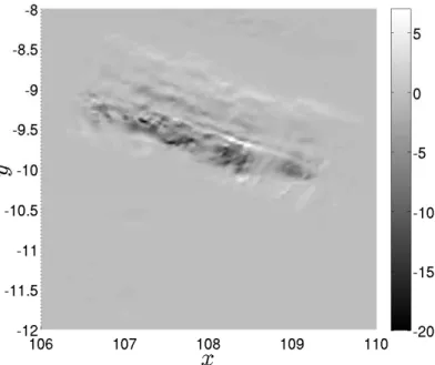
We begin our numerical investigations by quantifying the contribution of horizontal dis- placements into the sea bed deformation process. For this purpose we consider the differ- encedh(~x) between the deformed bottom under the action of only horizontal displacements in their steady state (t→+∞) and the initial configuration:
dh(~x) := h0 ~x+~u1,2(~x, t)|t→+∞
−h0(~x)
~max
x,t→+∞|u3(~x, t)| .
On Figure5we plot the quantitative effect of horizontal displacements relative to the maxi- mum vertical displacement max
~x,t→+∞|u3(~x, t)|. The computations performed showed that the maximum amplitude of the bottom variation due to the action of horizontal displacements reaches 21% of the maximum amplitude of the vertical displacement. In practice it means that locally (depending on the bathymetry shape and the slip distribution) we cannot completely neglect the effect of horizontal motion.
The next step consists in quantifying the impact of horizontal displacements onto free surface motion. We put six numerical wave gauges at the following locations: (a) (107.2◦,
−9.388◦), (b) (107.4◦, −9.205◦), (c) (107.6◦, −9.648◦), (d) (107.7◦, −9.411◦), (e) (108.3◦,
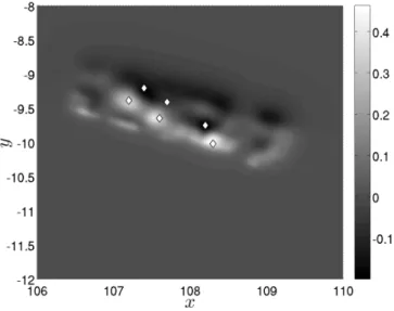
−10.02◦), (f) (108.2◦, −9.75◦). The locations of the wave gauges are represented by the symbol ⋄ on Figure 6 along with the static sea bed displacement. Wave gauges are inten- tionally put in places where the largest waves are expected.
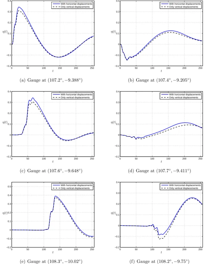
Numerical wave gauge records are presented in Figure 7. It can be seen that in most cases horizontal displacements lead to an increase in wave amplitude but not necessarily as
4Since we use a pseudo-spectral method, the convergence is expected to be exponential and this number of harmonics should be sufficient to capture all scales important for our study.
Figure 5. Contribution of horizontal displacements field into the sea bed deformation expressed in percentage of the maximum vertical displacement.
The grey color corresponds to negligible values while white and black zones show most important contributions.
Figure 6. Location of the six numerical wave gauges (indicated by the symbol ⋄) superposed with the steady state coseismic bottom displacement.
0 50 100 150 200 250
−0.2
−0.1 0 0.1 0.2 0.3 0.4
t η(t)
With horizontal displacements Only vertical displacements
(a) Gauge at (107.2◦,−9.388◦)
0 50 100 150 200 250
−0.2
−0.1 0 0.1 0.2 0.3 0.4
t η(t)
With horizontal displacements Only vertical displacements
(b) Gauge at (107.4◦,−9.205◦)
0 50 100 150 200 250
−0.2
−0.1 0 0.1 0.2 0.3 0.4
t η(t)
With horizontal displacements Only vertical displacements
(c) Gauge at (107.6◦,−9.648◦)
0 50 100 150 200 250
−0.2
−0.1 0 0.1 0.2 0.3 0.4
t η(t)
With horizontal displacements Only vertical displacements
(d) Gauge at (107.7◦,−9.411◦)
0 50 100 150 200 250
−0.2
−0.1 0 0.1 0.2 0.3 0.4 0.5
t η(t)
With horizontal displacements Only vertical displacements
(e) Gauge at (108.3◦,−10.02◦)
0 50 100 150 200 250
−0.2
−0.1 0 0.1 0.2 0.3 0.4
t η(t)
With horizontal displacements Only vertical displacements
(f) Gauge at (108.2◦,−9.75◦)
Figure 7. Free surface elevations computed numerically at six wave gauges located approximately in local extrema of the static bottom displacement.
The vertical axis is represented in meters and time is given in seconds. The black dashed line corresponds to the wave generated only by vertical dis- placements (incomplete generation) while the blue solid line takes also into account the horizontal displacements contribution (complete scenario). Note a change in vertical scale in Figure (e).
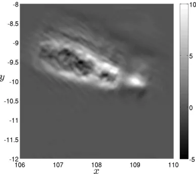
Figure 8. Relative difference between the free surface elevation at te = 220 seconds computed according to the complete ηc(~x, te) (with horizontal displacements) and incomplete ηi(~x, te) (only vertical component) tsunami generation scenarios. The vertical scale is given in percents of the maximum amplitude of the incomplete scenario — max
~
x ηi(~x, te).
it is shown in Figure7(f) (the last wave gauge located at (108.2◦,−9.75◦)). We investigated more thoroughly this question. Figure 8shows the relative difference between free surface elevations computed according to completeηh(~x, te) and incompleteη(~x, te) scenarios. More precisely, we plot the following quantity:
d(~x) := ηh(~x, te)−η(~x, te)
max~x |η(~x, te)| , te = 220s.
The time te = 220 s is chosen just when the bottom motion finishes and the wave enters in the free propagation regime. In Figure 8 the grey color corresponds to the zero value of the difference d(~x), while the white color shows regions where the wave is amplified by horizontal displacements by approximately 10%. On the contrary, black zones show an attenuation effect of horizontal sea bed motion (about −5%). Recall that all values are given in terms of the maximum amplitude max
~
x |η(~x, te)| percentage of the incomplete generation approach. Some correlation with the results presented in Figure 5 can be noticed.
Finally, we study the evolution of kinetic and potential energies during the tsunami gen- eration process described in Section2.2.1. Specifically we are interested in the contribution
0 50 100 150 200 250 0
5 10 15x 1011
t, s
Π(t),J
Potential energy
With horizontal displacements Only vertical displacements
(a) Potential energy Π(t), J
0 50 100 150 200 250
0 0.5 1 1.5 2 2.5 3 3.5
4x 10¹²
t, s
K(t),J
Kinetic energy
With horizontal displacements Only vertical displacements
(b) Kinetic energyK(t), J
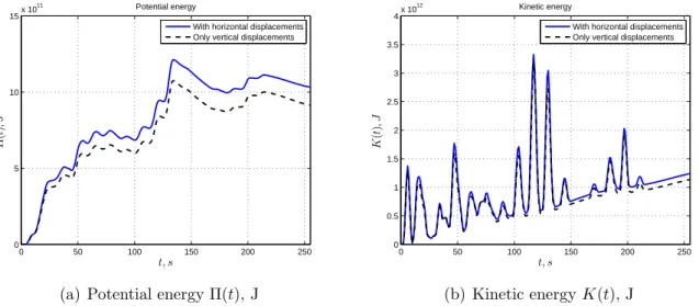
Figure 9. Energy evolution during our simulations in complete (blue solid line) and incomplete (black dotted line) scenarios. Note that scales are dif- ferent on left and right images.
of horizontal displacements into tsunami energy balance. Figure 9 shows the evolution of potential (9(a)) and kinetic (9(b)) energies in complete (blue solid line) and incomplete (black dashed line) scenarios. Consecutive peaks in the kinetic energy come from activation of new fault segments in accordance with the rupture propagation along the fault.
Despite some local attenuation effects of horizontal displacements on the free surface elevation, the complete generation scenario produces a tsunami wave with more important energy content. Namely, at the end of the simulation (T = 255 s) the total energy Π(T) + K(T) computed according to the complete scenario is equal to 2.27×10¹²J. The incomplete scenario leads to the total energy of 2.05×10¹² J. Consequently, horizontal displacements in our particular case of July 17, Java 2006 event contribute approximately 10% into the total tsunami energy value. This value is consistent with our previous results concerning the differences in wave amplitudes (see Figure8).
It is also interesting to compare the tsunami energy with energy of the underlying seismic event. USGS Energy and Broadband solution indicates that the radiated seismic energy of the Java 2006 earthquake is equal to 3.2×10¹⁴ J. Hence, according to our computations with the complete generation approach, about 0.71% of the seismic energy was transmitted to the tsunami wave. The ratio of the total tsunami and seismic radiated energies can be used as a measure of the tsunami generation efficiency of a specific earthquake.
This parameter can be also estimated for the great Sumatra-Andaman earthquake of December 26, 2004. The total energy of the Great Indian Ocean tsunami 2004 was esti- mated by T. Layet al. (2005) [LKA+05] to be equal to 4.2×10¹⁵J. According to the same USGS Energy and Broadband solution the radiated seismic energy was equal to 1.1×10¹⁷ J. Thus, the tsunamigenic efficiency of the Great Sumatra-Andaman earthquake is 3.8%
which is bigger than that of Java 2006 event but remains in the same order of magnitude
around 1%. It is probable that we do not still take into account all important factors in Java 2006 tsunami genesis.
4. Discussion and conclusions
In the present study the process of tsunami generation is further investigated. Main ingredients have already been presented in our previous study [DMG10]. Namely, the current tsunami genesis model relies on a combination of the finite fault solution [JWH02]
and recently proposed Weakly Nonlinear (WN) solver for the water wave problem with moving bottom [DMG10]. Consequently, in our model we incorporate recent advances in seismology and computational hydrodynamics.
This study is focused on the role of the horizontal displacements in the real world tsunami genesis process. By our intuition we know that a horizontal motion of the flat bottom will not cause any significant disturbance on the free surface. However, the real bathymetry is far from being flat. The question which arises naturally is how to quantify the effect of horizontal coseismic displacements during real world events?
The primary goal of this study was to propose relatively simple, efficient and accurate procedures to model tsunami generation process in realistic environments. Special emphasis was payed to the role of horizontal displacements which should be also taken into account.
Thus, the dynamics of horizontal coseismic displacements were reconstructed and their effect on free surface motion was quantified. The evolution of kinetic and potential energies were also investigated in our study. In the case of July 17, 2006 Java event our simulations indicate that 10% of the energy input can be seemingly ascribed to effects of the horizontal bottom motion.
The results presented in this study does not provide any evidence for the extreme runup values caused by July 17, 2006 Java tsunami [FKM+07], since but illustrate the proposed methodology on this important real world event. In our opinion the successful theory should incorporate various generation mechanisms.
Acknowledgement
D. Dutykh acknowledges the support from French Agence Nationale de la Recherche, project MathOcean (Grant ANR-08-BLAN-0301-01) and Ulysses Program of the French Ministry of Foreign Affairs under the project 23725ZA. The work of D. Mitsotakis was supported by Marie Curie Fellowship No. PIEF-GA-2008-219399 of the European Com- mission. French-Russian collabotation is supported by CNRS PICS project No. 5607.
L. Chubarov and Yu. Shokin acknowledge the support from the Russian Foundation for Basic Research under RFBR Project No. 10-05-91052 and from the Basic Program of Fundamental Research SB RAS Project No. IV.31.2.1.
We would like to thank Professors Didier Clamond and Fr´ed´eric Dias for very helpful discussions on numerical simulation of water waves. Special thanks go to Professor Costas Synolakis whose works on tsunami waves have also been the source of our inspiration.
References
[AJT+05] C.J. Ammon, C. Ji, H.-K. Thio, D. Robinson, S. Ni, V. Hjorleifsdottir, H. Kanamori, T. Lay, S. Das, D. Helmberger, G. Ichinose, J. Polet, and D. Wald. Rupture process of the 2004 Sumatra-Andaman earthquake.Science, 308:1133–1139, 2005.1
[AKLV06] C. J. Ammon, H. Kanamori, T. Lay, and A. A. Velasco. The 17 July 2006 Java tsunami earthquake.Geophysical Research Letters, 33:L24308, 2006.2,12
[BCD+09] S. Beisel, L. Chubarov, I. Didenkulova, E. Kit, A. Levin, E. Pelinovsky, Yu. Shokin, and M. Sladkevich. The 1956 Greek tsunami recorded at Yafo, Israel, and its numerical modeling.
Journal of Geophysical Research - Oceans, 114:C09002, 2009.7
[BCHK06] T. Baba, P.R. Cummins, T. Hori, and Y. Kaneda. High precision slip distribution of the 1944 Tonankai earthquake inferred from tsunami waveforms: Possible slip on a splay fault.
Tectonophysics, 426:119–134, 2006.7
[Ber70] E. Berg. Field survey of the tsunamis of 28 March 1964 in Alaska, and conclusions as to the origin of the major tsunami. Technical report, Hawaii Institute of Geophysics, University of Hawaii, Honolulu, 1970.3,4
[Bil05] R. Bilham. A flying start, then a slow slip.Science, 308:1126–1127, 2005.1
[BLM00] C. Bassin, G. Laske, and G. Masters. The current limits of resolution for surface wave tomog- raphy in North America.EOS Trans AGU, 81:F897, 2000.4
[CD10] D. Clamond and D. Dutykh. Practical use of variational principles for modeling water waves.
Submitted, http://arxiv.org/abs/1002.3019/, 2010.11
[CM85] R.R. Coifman and Y. Meyer. Nonlinear harmonic analysis and analytic dependence. Proc, symp. Pure Math, 43:71–78, 1985.10
[CS93] W. Craig and C. Sulem. Numerical simulation of gravity waves.J. Comput. Phys., 108:73–83, 1993.10
[CSS92] W. Craig, C. Sulem, and P.-L. Sulem. Nonlinear modulation of gravity waves: a rigorous approach.Nonlinearity, 5(2):497–522, 1992.10
[DB06] F. Dias and T.J. Bridges. The numerical computation of freely propagating time-dependent irrotational water waves.Fluid Dynamics Research, 38:803–830, 2006.10
[DD07a] F. Dias and D. Dutykh.Extreme Man-Made and Natural Hazards in Dynamics of Structures, chapter Dynamics of tsunami waves, pages 35–60. Springer, 2007.6,9
[DD07b] D. Dutykh and F. Dias. Viscous potential free-surface flows in a fluid layer of finite depth.C.
R. Acad. Sci. Paris, Ser. I, 345:113–118, 2007.9
[DD07c] D. Dutykh and F. Dias. Water waves generated by a moving bottom. In Anjan Kundu, editor, Tsunami and Nonlinear waves. Springer Verlag (Geo Sc.), 2007.2,4,6, 9
[DD09a] D. Dutykh and F. Dias. Energy of tsunami waves generated by bottom motion.Proc. R. Soc.
A, 465:725–744, 2009.3, 11
[DD09b] D. Dutykh and F. Dias. Tsunami generation by dynamic displacement of sea bed due to dip-slip faulting.Mathematics and Computers in Simulation, 80(4):837–848, 2009.2,4
[DDK06] D. Dutykh, F. Dias, and Y. Kervella. Linear theory of wave generation by a moving bottom.
C. R. Acad. Sci. Paris, Ser. I, 343:499–504, 2006.6,9
[DDZ08] F. Dias, A.I. Dyachenko, and V.E. Zakharov. Theory of weakly damped free-surface flows: a new formulation based on potential flow solutions.Physics Letters A, 372:1297–1302, 2008.9 [DKK08] A. I. Delis, M. Kazolea, and N. A. Kampanis. A robust high-resolution finite volume scheme for
the simulation of long waves over complex domains.Int. J. Numer. Meth. Fluids, 56:419–452, 2008.3
[DKM10] D. Dutykh, Th. Katsaounis, and D. Mitsotakis. Finite volume schemes for dispersive wave propagation and runup. Submitted to J. Comp. Phys., ( http://hal.archives-ouvertes.fr/hal- 00472431/ ), 2010.3
[DMG10] D. Dutykh, D. Mitsotakis, and X. Gardeil. On the use of finite fault solution for tsunami generation problem.Submitted (http://arxiv.org/abs/1008.2742), 2010.4,5,10, 11,13,18 [DP80] J. R. Dormand and P.J. Prince. A family of embedded Runge-Kutta formulae.J. Comp. Appl.
Math., 6:19–26, 1980.13
[DPD10] D. Dutykh, R. Poncet, and F. Dias. Complete numerical modelling of tsunami waves: gen- eration, propagation and inundation. Submitted, ( http://arxiv.org/abs/1002.4553 ), 2010.2, 3
[Dut07] D. Dutykh.Mathematical modelling of tsunami waves. PhD thesis, ´Ecole Normale Sup´erieure de Cachan, 2007.2,3, 6,9
[Dut09a] D. Dutykh. Group and phase velocities in the free-surface visco-potential flow: new kind of boundary layer induced instability.Physics Letters A, 373:3212–3216, 2009.9
[Dut09b] D. Dutykh. Visco-potential free-surface flows and long wave modelling.Eur. J. Mech. B/Fluids, 28:430–443, 2009.9
[FCKG05] D. Fructus, D. Clamond, O. Kristiansen, and J. Grue. An efficient model for threedimensional surface wave simulations. Part i: Free space problems.J. Comput. Phys., 205:665–685, 2005.
10,11
[FG07] D. Fructus and J. Grue. An explicit method for the nonlinear interaction between water waves and variable and moving bottom topography.J. Comp. Phys., 222:720–739, 2007.4
[FKM+07] H. M. Fritz, W. Kongko, A. Moore, B. McAdoo, J. Goff, C. Harbitz, B. Uslu, N. Kalligeris, D. Suteja, K. Kalsum, V. V. Titov, A. Gusman, H. Latief, E. Santoso, S. Sujoko, D. Djulka- rnaen, H. Sunendar, and C. Synolakis. Extreme runup from the 17 July 2006 Java tsunami.
Geophys. Res. Lett., 34:L12602, 2007.12,18
[FM09] D.R. Fuhrman and P.A. Madsen. Tsunami generation, propagation, and run-up with a high- order Boussinesq model.Coastal Engineering, 56(7):747–758, 2009.4
[GBAT06] E.L. Geist, S.L. Bilek, D. Arcas, and V.V. Titov. Differences in tsunami generation between the December 26, 2004 and March 28, 2005 Sumatra earthquakes.Earth Planets Space, 58:185–193, 2006.1,2,4
[GN07] P. Guyenne and D.P. Nicholls. A high-order spectral method for nonlinear water waves over moving bottom topography.SIAM J. Sci. Comput., 30(1):81–101, 2007.11
[Gus78] V.K. Gusiakov. Residual displacements on the surface of elastic half-space. In Conditionally correct problems of mathematical physics in interpretation of geophysical observations, pages 23–51, 1978.2
[Ham72] J.L. Hammack.Tsunamis – A Model of Their Generation and Propagation. PhD thesis, Cali- fornia Institute of Technology, 1972.6
[Ham73] J. Hammack. A note on tsunamis: their generation and propagation in an ocean of uniform depth. J. Fluid Mech., 60:769–799, 1973. W. M. Keck Laboratory of Hydraulics and Water Resources, California Institute of Technology, Pasadena.6,7
[Ima96] F. Imamura. Long-wave runup models, chapter Simulation of wave-packet propagation along sloping beach by TUNAMI-code, pages 231–241. World Scientific, 1996.3,4
[ISAL00] G.A. Ichinose, K. Satake, J.G. Anderson, and M.M. Lahren. The potential hazard from tsunami and seiche waves generated by large earthquakes within Lake Tahoe, California-Nevada.Geo- phys. Res. Lett., 27:1203–1206, 2000.2
[IYO06] F. Imamura, A.C. Yalciner, and G. Ozyurt.Tsunami modelling manual, April 2006.4
[Ji06] C. Ji. Preliminary result of the 2006 July 17 magnitude
7.7 - south of Java, Indonesia earthquake. Technical report, http://neic.usgs.gov/neis/eq_depot/2006/eq_060717_qgaf/neic_qgaf_ff.html, 2006.
4,6,12
[JS93] J.M. Johnson and K. Satake. Source parameters of the 1957 Aleutian earthquake from tsunami waveforms.Geophysical Research Letters, 20:1487–1490, 1993.1
[JWH02] C. Ji, D. J. Wald, and D. V. Helmberger. Source description of the 1999 Hector Mine, California earthquake; Part I: Wavelet domain inversion theory and resolution analysis.Bull. Seism. Soc.
Am., 92(4):1192–1207, 2002.4, 18
[Kaj63] K. Kajiura. The leading wave of tsunami.Bull. Earthquake Res. Inst., Tokyo Univ., 41:535–571, 1963.2
[Kaj70] K. Kajiura. Tsunami source, energy and the directivity of wave radiation. Bull. Earthquake Research Institute, 48:835–869, 1970.4
[Kan70] H. Kanamori. The Alaska earthquake of 1964: Radiation of long-period surface waves and source mechanism.Journal of Geophysical Research, 75(26):5029–5040, 1970.1
[KCY07] D.-H. Kim, Y.-S. Cho, and Y.-K. Yi. Propagation and run-up of nearshore tsunamis with HLLC approximate Riemann solver.Ocean Engineering, 34:1164–1173, 2007.3
[KDD07] Y. Kervella, D. Dutykh, and F. Dias. Comparison between three-dimensional linear and non- linear tsunami generation models.Theor. Comput. Fluid Dyn., 21:245–269, 2007.4, 6,9,11 [Lam32] H. Lamb.Hydrodynamics. Cambridge University Press, 1932.8
[Lan96] J.F. Lander. Tsunamis affecting Alaska 1737 – 1996.U.S. Department of Commerce, National Oceanic and Atmospheric Administration, 31:195, 1996.2
[LKA+05] T. Lay, H. Kanamori, C. J. Ammon, M. Nettles, S. N. Ward, R. C. Aster, S. L. Beck, S. L.
Bilek, M. R. Brudzinski, R. Butler, H. R. DeShon, G. Ekstrom, K. Satake, and S. Sipkin. The great Sumatra-Andaman earthquake of 26 December 2004.Science, 308:1127–1133, 2005.1,17 [Mei94] C.C. Mei.The applied dynamics of ocean surface waves. World Scientific, 1994.8
[Min36] R. D. Mindlin. Force at a point in the interior of a semi-infinite medium.Physics, 7:195–202, 1936.6
[Mit09] D.E. Mitsotakis. Boussinesq systems in two space dimensions over a variable bottom for the generation and propagation of tsunami waves.Math. Comp. Simul., 80:860–873, 2009.3 [MS67] L. Mansinha and D. E. Smylie. Effect of earthquakes on the Chandler wobble and the secular
polar shift.J. Geophys. Res., 72:4731–4743, 1967.2,6
[MS71] L. Mansinha and D. E. Smylie. The displacement fields of inclined faults. Bull. Seism. Soc.
Am., 61:1433–1440, 1971.2, 6
[OK06] A. Ozgun Konca. Preliminary result 06/07/17 (Mw 7.9) , Southern Java earthquake. Technical report, http://www.tectonics.caltech.edu/slip_history/2006_s_java/s_java.html, 2006.12
[Oka85] Y. Okada. Surface deformation due to shear and tensile faults in a half-space.Bull. Seism. Soc.
Am., 75:1135–1154, 1985.2, 5
[Oka92] Y. Okada. Internal deformation due to shear and tensile faults in a half-space. Bull. Seism.
Soc. Am., 82:1018–1040, 1992.2, 5
[OTM01] T. Ohmachi, H. Tsukiyama, and H. Matsumoto. Simulation of tsunami induced by dynamic displacement of seabed due to seismic faulting.Bull. Seism. Soc. Am., 91:1898–1909, 2001.2 [Pre65] F. Press. Displacements, strains and tilts at tele-seismic distances.J. Geophys. Res., 70:2395–
2412, 1965.6
[RLF+08] A. B. Rabinovich, L. I. Lobkovsky, I. V. Fine, R.E. Thomson, T. N. Ivelskaya, and E. A.
Kulikov. Near-source observations and modeling of the Kuril Islands tsunamis of 15 November 2006 and 13 January 2007.Adv. Geosci., 14:105–116, 2008.2
[SB06] C.E. Synolakis and E.N. Bernard. Tsunami science before and beyond Boxing Day 2004.Phil.
Trans. R. Soc. A, 364:2231–2265, 2006.1
[SF09] T. Saito and T. Furumura. Three-dimensional tsunami generation simulation due to sea-bottom deformation and its interpretation based on the linear theory.Geophys. J. Int., 178:877–888, 2009.2,11
[SFZ+08] Y.T. Song, L.-L. Fu, V. Zlotnicki, C. Ji, V. Hjorleifsdottir, C.K. Shum, and Y. Yi. The role of horizontal impulses of the faulting continental slope in generating the 26 December 2004 tsunami.Ocean Modelling, 20:362–379, 2008.4, 7
[Ste05] D.J. Stevenson. Tsunamis and earthquakes: What physics is interesting? Physics Today, June:10–11, 2005.2
[Sto58] J.J. Stoker.Water waves, the mathematical theory with applications. Wiley, 1958.8 [Tan86] M. Tanaka. The stability of solitary waves.Phys. Fluids, 29(3):650–655, 1986.11
[TG97] V.V. Titov and F.I. Gonz´alez. Implementation and testing of the method of splitting tsunami (MOST) model. Technical Report ERL PMEL-112, Pacific Marine Environmental Laboratory, NOAA, 1997.4
[THT02] M.I. Todorovska, A. Hayir, and M.D. Trifunac. A note on tsunami amplitudes above submarine slides and slumps.Soil Dynamics and Earthquake Engineering, 22:129–141, 2002.6
[TIM+95] Y. Tsuji, F. Imamura, H. Matsutomi, C.E. Synolakis, P.T. Nanang, Jumadi, S. Harada, S.S.
Han, K. Arai, and B. Cook. Field survey of the East Java earthquake and tsunami of June 3, 1994.Pure Appl. Geophys., 144:839–854, 1995.2
[TS96] Y. Tanioka and K. Satake. Tsunami generation by horizontal displacement of ocean bottom.
Geophysical Research Letters, 23:861–864, 1996.3, 4,7
[TT01] M. I. Todorovska and M. D. Trifunac. Generation of tsunamis by a slowly spreading uplift of the seafloor.Soil Dynamics and Earthquake Engineering, 21:151–167, 2001.4,6
[Vol07] V. Volterra. Sur l’´equilibre des corps ´elastiques multiplement connexes.Annales Scientifiques de l’Ecole Normale Sup´erieure, 24(3):401–517, 1907.5
[Whi99] G.B. Whitham.Linear and nonlinear waves. John Wiley & Sons Inc., New York, 1999.8 [WIS05] K.T. Walker, M. Ishii, and P.M. Shrearer. Rupture details of the 28 March 2005 Sumatra Mw
8.6 earthquake imaged with teleseismic P waves.Geophysical Research Letters, 32:24303, 2005.
1
[Zak68] V.E. Zakharov. Stability of periodic waves of finite amplitude on the surface of a deep fluid.J.
Appl. Mech. Tech. Phys., 9:1990–1994, 1968.10
LAMA, UMR 5127 CNRS, Universit´e de Savoie, Campus Scientifique, 73376 Le Bourget- du-Lac Cedex, France
E-mail address: Denys.Dutykh@univ-savoie.fr URL:http://www.lama.univ-savoie.fr/~dutykh/
UMR de Math´ematiques, Universit´e de Paris-Sud, Bˆatiment 425, P.O. Box, 91405 Orsay, France
E-mail address: Dimitrios.Mitsotakis@math.u-psud.fr URL:http://sites.google.com/site/dmitsot/
Institute of Computational Technologies, Siberian Branch of the Russian Academy of Sciences, 6 Acad. Lavrentjev Avenue, 630090 Novosibirsk, Russia
E-mail address: chubarov@ict.nsc.ru URL:http://www.ict.nsc.ru/
Institute of Computational Technologies, Siberian Branch of the Russian Academy of Sciences, 6 Acad. Lavrentjev Avenue, 630090 Novosibirsk, Russia
E-mail address: shokin@ict.nsc.ru URL:http://www.ict.nsc.ru/
![Figure 2. Trigonometric dynamic scenario for t r = 1 s (see J. Hammack (1973), [Ham73]).](https://thumb-eu.123doks.com/thumbv2/1bibliocom/472614.75638/8.892.273.622.148.434/figure-trigonometric-dynamic-scenario-j-hammack-1973-ham73.webp)