MODELING THE ASIAN TSUNAMI EVOLUTION AND PROPAGATION WITH A NEW GENERATION MECHANISM AND A NON-LINEAR DISPERSIVE WAVE
MODEL
Paul C. Rivera PEERS Coastal Research, Antipolo City, PHILIPPINES
ABSTRACT
A common approach in modeling the generation and propagation of tsunami is based on the assumption of a kinematic vertical displacement of ocean water that is analogous to the ocean bottom displacement during a submarine earthquake and the use of a non-dispersive long-wave model to simulate its physical transformation as it radiates outward from the source region. In this study, a new generation mechanism and the use of a highly-dispersive wave model to simulate tsunami inception, propagation and transformation are proposed. The new generation model assumes that transient ground motion during the earthquake can accelerate horizontal currents with opposing directions near the fault line whose successive convergence and divergence generate a series of potentially destructive oceanic waves. The new dynamic model incorporates the effects of earthquake moment magnitude, ocean compressibility through the buoyancy frequency, the effects of focal and water depths, and the orientation of ruptured fault line in the tsunami magnitude and directivity.
For tsunami wave simulation, the nonlinear momentum-based wave model includes important wave propagation and transformation mechanisms such as refraction, diffraction, shoaling, partial reflection and transmission, back-scattering, frequency dispersion, and resonant wave-wave interaction. Using this model and a coarse-resolution bathymetry, the new mechanism is tested for the Indian Ocean tsunami of December 26, 2004. A new flooding and drying algorithm that consider waves coming from every direction is also proposed for simulation of inundation of low-lying coastal regions.
It is shown in the present study that with the proposed generation model, the observed features of the Asian tsunami such as the initial drying of areas east of the source region and the initial flooding of western coasts are correctly simulated. The formation of a series of tsunami waves with periods and lengths comparable to observations are also well simulated with the new generation model. Furthermore, the shoaling behavior of the tsunami waves during flooding of dry land was also simulated by the new run-up algorithm. Finally, the new generation and propagation models can explain the combined and independent effects of various factors in tsunami generation and transformation taking into consideration the properties of the ocean and the geologic disturbance.
1.0 INTRODUCTION
Tsunami modeling has always been traditionally undertaken using the shallow water wave equations which are non-frequency dispersive long wave equations. However, recently observed data from the Indian Ocean Tsunami of Dec 26, 2004 using satellite altimetry data that were subject to wavelet analysis by Kulikov (2005) found that the tsunami waves were highly dispersive. It is therefore the aim of this study to develop and implement a dispersive wave model to simulate the propagation and transformation of the tsunami that occurred in the Indian Ocean. In addition, a new generation mechanism that is based on the assumption that currents were induced during the earthquake is also proposed in this study.
The difficulty in correctly simulating tsunamis lies in the fact that they are forced quasi-infra-gravity waves whose characteristic length and period occur in between short gravity wind-waves and long-gravity waves such as tides or storm surges so that they can not be fully described by conventional long wave models. Being a forced wave that depends on the characteristics of the disturbing force, a tsunami wave does not behave exactly as a long wave nor a short wave, but behaves as an intermediate wave that is modified and transformed by the oceanic and seabed properties as it travels away from the generation area.
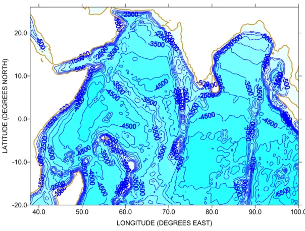
In testing the present dispersive model and a new generation mechanism, the present study makes use of the coarse-resolution bathymetric information from NOAA-NGDC (ETOPO-5 which was aggregated further to reduce computational time). The study area with bathymetric contours (in meters) is shown in Figure 1.
40.0 50.0 60.0 70.0 80.0 90.0 100.0
LONGITUDE (DEGREES EAST) -20.0
-10.0 0.0 10.0 20.0
L
A
TITU
D
E
(DEGR
EES
NO
R
T
H)
Figure 1. Bathymetric contours (m) within the study area.
2.0 PROPOSED GENERATION MECHANISM
Tsunami occurrence had been documented during submarine earthquakes, volcanic island eruptions, and landslides. Even when an earthquake epicenter is inland or at sea, some tsunami had also been observed. It is therefore appropriate to find a better generation mechanism other
than the conventional approach of determining the ocean surface displacement as a result of seabed motion.
The present generation model can be explained in terms of balance of forces. During a submarine earthquake, an upward force or pressure is exerted in the ocean column by the seabed (Figure 2). Similar to atmospheric pressure effect, this produces a horizontal pressure gradient which should accelerate currents opposite to the direction of the applied pressure gradient force (i.e. -ρ−1∇ =Pe ax, where ρ is water density, Pe is seabed pressure and ax is
horizontal acceleration). It is postulated that a tsunami may occur if the prevailing downward force or pressure of the ocean column is exceeded by the pressure or force exerted by the seabed. Furthermore, it is also proposed that a seismic-induced pressure gradient force would accelerate currents across the fault. That is, a cross-fault current is generated as shown in Figure 2. The slope of the seabed here may play an important role as it strongly affects the magnitude and direction of the induced currents. In the case of the Asian Tsunami, the increasing water depths towards the west could mean that westerly currents are generated by the quake.
P(e)
Fault
Ocean column u(x,y,t)
cross-fault current
Figure 2. Schematic illustration of the proposed tsunami generation model.
Ocean surface
The figure above implies that if the earthquake moment magnitude is high enough, the pressure exerted at the ocean bottom may exceed the pressure exerted by the atmosphere and the water column. This in turn produces an excess pressure whose horizontal gradient (i.e. the pressure gradient force), creates a horizontal acceleration of currents near the fault-line. The impulsive momentum of these horizontal currents and their succeeding convergence and divergence can produce a series of waves that radiates away from the source.
The tsunami generation mechanism that is proposed here may be used to study the waves generated during volcanic eruptions or landslides. During these geologic events, ground accelerations can produce opposing horizontal ocean currents whose successive divergence and convergence can generate potentially destructive tsunami waves. It is assumed that the ocean currents produced by the ground motion oscillates at a frequency that is dependent on the local water depth and the gravitational acceleration. The oceanic currents produced during the submarine earthquake oscillate in time t according to:
(
, ,)
z hsin(
u x y t N t ts
κα ∆ ω
=
∆
)
(1)where u(x,y,t) is the magnitude of the induced horizontal current (m/s), is a non-dimensional tuning parameter (= 0.5 in the present study), α is a variable that include factors related to both the seismic disturbance and the ocean column, N
κ
frequency of the ocean column), h
s ∆
∆ is the bathymetric slope of the disturbed seabed, and ω is
a local current frequency given by ω=2 /π Tc. Here, Tc is the period of current oscillation
which is given by h g/ / 2 in which h is the water depth and g is gravitational acceleration. After a long series of numerical experiments and making use of the Buckingham pi-theorem, the dimensional parameter α is found to be;
(
)
1 3
1 10
4
w M
g D h
α
ρ υ
=
+
(2)
in which Mw is the moment magnitude of the earthquake, ω is the local frequency of current
oscillation, D is the focal depth of the earthquake, and ν is the kinematic viscosity of seawater. The moment magnitude of the earthquake is an important parameter here as higher Mw values
mean higher current accelerations and current velocity generated. The estimated value of α is similar to an induced horizontal motion of water above the disturbed seabed. In Equation 2, the focal depth increases when the earthquake epicenter is not submarine (e.g. when located inland) giving rise to relatively lower value of α as itis inversely proportional to D. In such a
case where the epicenter is located inland, the focal depth D becomes D= Dv2 +Dh2 where
Dv is the actual focal depth directly beneath the epicenter and Dh is the horizontal distance
from the epicenter to the ocean water. This case implies relatively lower magnitudes of currents produced by the earthquake and lower tsunami wave heights as well, given all earthquake and ocean parameters constant.
The present model supports the observation that tsunamis can be generated by both submarine and inland shallow-focus earthquakes near deep maritime environments. It is hypothesized however, that when prevailing oceanic currents interfere with the seismic-induced ocean currents in a deep-sea environment where bathymetric slope is large, an abnormally high tsunami can be generated (as supported by the proposed generation model). The Papua New Guinea earthquake of 1998 could be an example of this observation.
The period of current oscillation produced during and after the earthquake is dependent on the square root of the water depth divided by the gravitational acceleration. In the Indian Ocean source region of the December 2004 earthquake, this takes about 10 seconds assuming an ocean depth of about 4000 m. It can be seen from the continuity equation that shallow coastal areas do not favor the generation of strong currents (and consequently high waves) even during strong earthquakes. The difference between the new model from the conventional kinematic model is that the dynamic motion of the ocean column can now be simulated by virtue of the induced currents. When the seabed disturbance sets in, the seawater responds almost immediately as the rupture velocity goes at an enormous speed (= 2 km/s). The proposed tsunami generation model assumes that the ocean currents oscillates in time with a maximum duration equal to the inverse of the buoyancy frequency (T~ 2π/Nz). The buoyancy
frequency is considered an important hydrodynamic factor in the new generation model. Nz is
the frequency of oscillation for a water mass that is displaced vertically upwards during seabed displacement. It is dictated by the vertical stability and compressibility of the ocean column and is given by;
2 2
z
o
g g
N
c z
ρ ρ
∂
= −
∂ (3)
Here, c is the speed of sound in seawater (about 1485 m/s), ρo is the reference density (about
1025 kg/m3). Assuming a -3 kg/m3 density difference from surface to bottom in a 4 km ocean depth, this gives a buoyancy frequency Nz = 0.00713 s-1. Given all earthquake parameters
constant, it can be seen from Equation (1) that the stability of the water column can increase the current acceleration or velocity (and consequently, the wave heights) if the vertical stratification of the water column is stable with negative vertical density gradient giving Nz a
higher magnitude. The effect of wave amplification due to ocean compressibility has been suggested by Hunt (1993).
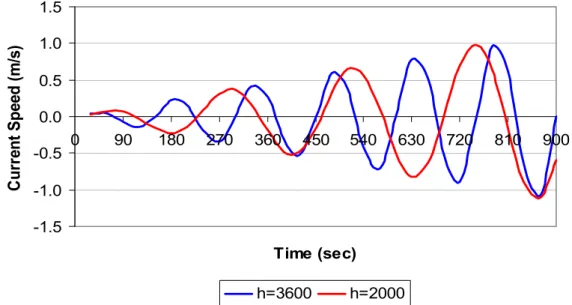
A time-series plot of the induced horizontal currents within the source area is shown in Figure 3. In general, spatially non-uniform current (and wave) patterns would develop due to non-uniformity of ocean bottom and the pressure gradient forces acting in the water column. The spatial variation of current in the present formula is assumed to depend only on the variation of depth within the source region. Due to bathymetric changes, divergence and convergence of currents may also occur giving a turbulent and complex current velocity field in the source region. It is hypothesized that these currents should continue to oscillate even after cessation of the fault line rupture until dissipated by friction.
-1.5 -1.0 -0.5 0.0 0.5 1.0 1.5
0 90 180 270 360 450 540 630 720 810 900
Time (sec)
Cu
rre
n
t S
p
e
e
d
(
m
/s
)
h=3600 h=2000
Figure 3. Current oscillations generated in a water depth of 3.6 km and 2 km during a submarine earthquake. The induced ocean currents can produce a series of
potentially destructive tsunami waves.
Depending on the magnitudes of the currents generated and the overall physical oceanographic characteristics of the source region and its vicinity, these currents can become transoceanic and can generate a series of destructive waves that can travel long distances away from the source region. The horizontal currents produced by the seismic disturbance should be spatially non-uniform and not constant at the opposite sides of the ruptured fault since the water depth and the seabed pressure vary horizontally. The proposed formula gives an estimate of the spatial and temporal variation of the ocean currents within the source region. Assuming an earthquake moment magnitude Mw = 9.1, the maximum current magnitude
estimated by the present model was about 2 m/s. It is assumed that after the time period T, the induced-current will continue to oscillate but decreases in time opposite to the increasing current shown in Figure 3.
the ocean column opposite to the atmospheric (and hydrostatic) pressure gradient force. The recently observed ‘dead zone’ along the tsunami source region west of Sumatra is most likely caused by the induced strong oceanic currents near the seabed and not directly by the oceanic waves. This is because the water is just too deep in the area for even an abnormally high offshore tsunami to impart a considerable wave action at the seabed.
3.0 TSUNAMI MODELING WITH A NON-LINEAR DISPERSIVE LONG WAVE MODEL
As altimeter data from satellites showed that the Indian Ocean tsunami was highly dispersive, it is therefore appropriate to use a dispersive long-wave model. This study differs from previous modeling studies conducted by various authors in that a dispersive wave model was used in the open ocean instead of the conventional non-dispersive long-wave model.
Assuming that water density does not change with time, the partial differential equation describing the time-dependent variation of the surface wave heights in the ocean area of interest is given by the modified mass continuity equation:
(
)
(
)
0
u h u h
p
t x y
∂ ζ ∂ ζ
∂ ζ
∂ ∂ ∂
+ +
+ + = (4)
where p is the porosity, ζ is the wave height, t is time, and x and y are coordinate axes in the Cartesian system, u and v are the mean components of the wave-induced flow in the x and y-axes respectively, τs is the wind stress acting over the sea surface, ρ is the sea water density, h
is the total water depth, and ho is the still water level. Similar to the dispersive wave model of
Madsen and Sorensen (1992), the porosity factor p is included for the simulation of partial wave reflection and transmission. This time-dependent equation allows for the determination of the temporal as well as spatial variation and evolution of the wave height due to the divergence (and convergence) of the horizontal currents produced by an applied disturbance of various origins (e.g. seismic, atmospheric, landslides etc).
The difficulty in modeling tsunami can be due to the fact that they are intermediate, quasi-infra-gravity waves, having the combined characteristics of long and short ocean waves. As initiated by previous authors (e.g. Koutitas and Laskaratos 1988, Pedersen et al. 2005), the initial idea in the present study was to seek a combination between a dispersive and non-dispersive model. The non-non-dispersive model may be applied in the open ocean while the dispersive model could be applied in shallow coastal areas to determine the transformation of the waves as they travel from deep to shallow waters. Incidentally, the non-linear dispersive momentum equations originally proposed by Peregrine (1967) and Wu (1981) for the study of long waves in oceans and beaches were modified and applied in this study. In combination with a simple periodic current induced by a seismic disturbance, the simple dispersive model worked. Various combinations of momentum terms such as those proposed by Madsen and Sorensen (1992) were tried. Eventually, the momentum equations were simplified due to negligible effect of some higher-order terms. The effect of ocean baroclinicity and compressibility is included by using a modified pressure gradient force. The modified momentum conservation equations for dispersive long gravity waves take the non-linear form:
( )
2 2 2 22 2 2
2 2
2 3 3 2 2 2 2
2 2
3 2
sx
z h
o o o o o
o o
h u u v
u u u u u
p u v pfv p g p N k p
t x y x x h h x y
h u v h h u h u v h v
p p ph ph
x t x y t x t x x t y t y x t
ζ
ζ τ υ
ρ ∂ + ∂ + ∂ + ∂ = − ∂ − + − + ∂ +∂ ∂ ∂ ∂ ∂ ∂ ∂ ∂ ∂ ∂ ∂ ∂ ∂ ∂ ∂ ∂ ∂ + + + + + + ∂ ∂ ∂ ∂ ∂ ∂ ∂ ∂ ∂ ∂ ∂ ∂ ∂ ∂ ∂ (5)
( )
2 2 2 22 2 2
2 2
2 3 3 2 2 2 2
2 2
3 2
sy
z h
o o o o o
o o
h v u v
v v v v v
p u v pfu p g p N k
t x y y y h h x y
h v u h h v h v u h u
p p ph ph
y t x y t y t y y t x t x y t
ζ
ζ τ υ
ρ
∂ +
∂ ∂ ∂ ∂ ∂ ∂
+ + = − − − + − + +
∂ ∂ ∂ ∂ ∂ ∂ ∂
∂ ∂ ∂ ∂ ∂ ∂ ∂ ∂ ∂
+ + + + + +
∂ ∂ ∂ ∂ ∂ ∂ ∂ ∂ ∂ ∂ ∂ ∂ ∂ ∂ ∂
(6)
where u and v are the depth-averaged wave-induced flow components in the x and y-axes respectively, p is a porosity factor that allows for partial reflection and transmission of waves, f
is the latitude-dependent Coriolis parameter, g is the gravitational acceleration, Nz is the
buoyancy (or Brunt-Vaisalla) frequency, k is a frictional resistance coefficient, and υh is the
horizontal eddy viscosity coefficient. The total water depth h is the sum of the still water depth
ho and the surface wave height ζ. As these equations represent a balance of forces in the
ocean, they are useful in dealing with non-linear dispersive long and intermediate waves in both deep and shallow coastal waters. In the present study, these dispersive wave equations are applied in both deep oceanic waters and shallow coastal waters. With the addition of dynamic pressure, wind effect, and horizontal viscosity, they represent the modified two-dimensional dispersive long-wave equations in oceans and coastal waters. The eight terms to the right of the momentum equations are considered important as they describe the diffusive effect of sloping ocean bottom. They also allow lower frictional effect where high friction often obliterates the real numerical solution by unnecessary damping of the resulting current velocity field. The last two terms are deep water terms and their effects are also small but considered here to represent the propagation of the tsunami waves from deep to shallow waters. Villenueve and Savage (1993) derived a more sophisticated momentum equation taking into consideration the bed motion. The present model assumes that the sea bed is stationary and it is the ocean column that moves in a dynamic fashion during and after the seismic disturbance.
The wind stress effect can be necessary to include the contribution of the wind energy in the horizontal momentum dispersion and hence in the long-distance propagation of the tsunami waves. The presence of the wind can be seen in an increased horizontal currents and the interaction between the wind-driven currents and the waves may be important during a tsunami occurrence. The wind stress terms can be estimated from quadratic stress formulas.
It can be seen that the pressure terms in the momentum equations consist of the sum of the hydrostatic and dynamic pressures due to a barotropic and a baroclinic ocean. This is considered important in geophysical flows with a considerable influence of vertical stability and vertical acceleration as could be the case during a tsunami.
The present wave model considers the effect of the tide by assuming that the water level periodically increase and decrease during high and low tide episodes. In coastal seas, the tide modifies the initial depth distribution and it could be a substantial fraction of the water depth in shallow areas. Waves propagating in shallow near-shore regions are thus affected by the temporal variation of the water depth introduced by the tide. The tidal current can therefore have a substantial effect on the tsunami wave propagation.
The non-dimensional bottom frictional resistance k is normally taken as constant with values ranging from 0.001-0.01. The lower limit was used in the present modeling study. The use of a Chezy or Manning formula for the bottom friction coefficient is also possible but the use of a constant coefficient is recommended in the present study as the wave run-up appears to be slightly attenuated with the former formulas.
The horizontal eddy viscosity is also included in this study and is parameterized using the Smagorinsky turbulence scale approach and the use of a constant eddy viscosity has been avoided. Here, horizontal viscosity is dependent on the gradient of the horizontal velocity components as in:
1/ 2
2 2
2
1 2
h
u v u v
A
x y x y
ν =υ ∂ + ∂ + ∂ +∂
∂ ∂ ∂ ∂
(7)
where υ is constant (0.01-0.5) and A is the area of a grid element. The present model uses a value of 0.05.
The effect of the earth’s rotation (e.g. Coriolis force) on the waves is also considered in the present study by including it in the momentum equations. In higher latitudes, the Coriolis force may have a significant effect especially when horizontal currents are strong and may therefore affect the tsunami waves as they travel away from the source region.
3.1 NUMERICAL SOLUTION AND MODEL IMPLEMENTATION
As the high-order dispersive terms in the momentum equations require a lot of transformation and complexity in the numerical solution, a rectangular coordinate system with square grid cells was used to simplify the solution of the coupled partial differential equations. The effect of the deep water terms (e.g. last 2 terms to the right of the momentum equations) may be negligible in deep ocean calculations but could be important in shallow waters. Therefore, it is recommended to retain the same number of terms in the momentum equations as they represent a balance of forces which should be applicable in both deep and shallow water domains.
For the simulation of the wave and tide processes, a Fourier series describing the tide variation in the computational area of interest has been implemented. The tide contributes much to the total water level especially in shallow areas. The contribution of the tide in the tsunami run-up can be very significant especially during high tidal phase. To include the tidal effect to the water depth, the Fourier series below was used.
1
cos( )
n
t o i i i
i
a a t
ζ ω φ
=
= +
∑
− (8)where ao is the mean amplitude of the tide level, ai is the amplitude, ωi is the frequency and Φi
is the phase of the ith tidal constituent. This tidal height ζt,is just added in the present study to
the total water depth h during the period of simulation. The four major tidal constituents namely O1, K1, M2 and S2 tides are included in the second term in the right-hand side of this
equation.
The numerical solution of the dispersive wave equations is based on an explicit finite difference scheme with the unknown variables staggered in space using the Arakawa C-Grid. The variables are solved with the wave height and water depth at the center of a grid cell. The depth-averaged current component in the x-axis is located at the center of a y-directed side (left and right of the grid mesh) and the current component in the y-axis is located at the center of an x-directed side. To simplify the finite differentiation of the momentum and continuity equations, the grid distance was assumed equal in the x and y-directions (∆x = ∆y = 30 min). In this space-staggered grid, the first order space derivatives are solved using high-order finite differences as in Kowalik (2003) given by
(
xx = i − i + i − i ∆
∂ ∂
+ −
−2 27η 1 27η η 1 /24
η
)
η
(9)
where η is the unknown variable (e.g. currents or waves).
The numerical integration proceeds from the calculation of the continuity equation and the specification of the open boundary condition. Here, the first-order spatial derivatives are solved using Equation 9. Using the newly computed wave height, the momentum equations are solved. Here, the u-component of the flow is solved throughout the computational domain using a second order upstream numerical scheme for the advective terms as proposed by Stelling (1984) and Kowalik (2003). The calculation of the earthquake-induced currents from Equation 1 is done after the u-component of currents is computed. After this, the calculation of the v-component of the current using the same second order upstream scheme for the advective terms follows. The pressure gradient terms (i.e. sum of barotropic and baroclinic pressures) and the horizontal bathymetric gradient of the deep-water terms in the momentum equations are also solved using high-order finite differences as in Equation 9. Filtering of computed velocity fields as in Kowalik (2003) was also carried out with a smoothing coefficient of 0.005. For boundary conditions, only wave height is prescribed. Here, wave heights in all the open ocean boundaries of the computational domain were treated with a pseudo-implicit form of the Orlanski Radiation condition described in literature (Rivera 1997). No special control mechanism is implemented near land and water boundaries as the proposed flooding and drying algorithm (described below) automatically computes waves and currents as long as there is water in grid cells of interest.
3.2 FLOODING ALGORITHM AND RUN-UP MODEL
The flooding and drying of low-lying areas is considered a difficult modeling problem. Together with the tsunami propagation from offshore to near-shore areas, inundation of dry land makes tsunami modeling an exceedingly difficult hydrodynamic problem (Beikae 2001). The succeeding run-down and periodic exposure of low-lying areas is less complicated to model numerically.
To handle the run-up and run-down problem, a simple computational algorithm of flooding and drying was developed and implemented in this study. Whenever the water depth is positive (i.e. greater than zero), the continuity and momentum equations area solved. The inclusion of the eight terms to the right of the momentum equations is shown to be very important in the numerical solution of the model equations. In the solution of the non-dispersive long-wave equations, the bottom frictional terms may lead to overflow of numerical solutions if the water depth is too low. However, with the inclusion of this slope-term, there is no associated over-flow problem in the momentum equations as long as the water depth is greater than zero. After successively computing for the wave heights and current components, the new water depth is updated (i.e. h = ho + ζ). Initially, grid cells which are dry (e.g. land
areas) have negative values determined by the height of the land above sea level. On the other hand, wet areas (e.g. ocean areas) have positive depths. For all grid points with non-zero wave height and positive depth, a counting index equal to 1.0 is assigned. On the other hand, all dry points (e.g. grid cells without water) are assigned a counting index of 0. During wave run-up onto dry land, the water depth is calculated using h = ho + ζbar where ζbar is the sum of all
surrounding non-zero wave heights divided by the sum of the counting indices. Here, when all surrounding grid cells have non-zero wave heights (i.e. all wet), ζbar is the average of 8 (and
surrounding cells with non-zero wave heights. When the new depth is positive, it will be considered in the next series of computations of the continuity equation. For the momentum equations, calculation of the u-component will proceed if hi,j and hi+1,j are greater than zero
(e.g. both adjacent grid points along x-direction are wet). In the same manner, calculation of the v-component will proceed if hi,j and hi, j+1 are greater than zero (e.g. both adjacent grid
points along y-direction are wet).
If the next grid cell is still dry during inundation (i.e. h is still negative), it will assume that new negative value and will not be considered in the next series of computation until it becomes wet or positive. However, it should be noted here that in these areas where the water flow is impeded by high grounds, the wave height can grow tremendously due to the associated strong spatial gradient in the horizontal currents during a tsunami approach to the shore. This shoaling behavior of the wave is reproduced by the present run-up algorithm by using a fine resolution small-scale model with a grid-distance of 150 m. The new flooding and run-up algorithm therefore requires accurate information about the topographic and bathymetric characteristics of flood-prone areas. Where inundation is expected to be far inland, the model grid should encompass all vulnerable low-lying areas with a very high resolution in space. With the present algorithm, the whole water-land area is part of the computational domain and does not require a moving boundary condition. Setting of a zero-normal velocity at high grounds is set automatically only from knowledge of the total water depth.
4.0 RESULTS AND DISCUSSION
In its numerical implementation, Equation 1 is applied from longitude 91.5 º E – 93 º E and latitude 2 º N -11 º N approximating water motion within the source region throughout the assumed period of oscillation T (14.68 min). It should be noted that in the present modeling study, a north-south orientation of the affected oceanic column was chosen to simplify the source specification. A curved source region similar in orientation to the ruptured fault can be assumed in future studies. After the quake, the currents are assumed to increase periodically. After the time duration T, the already accelerated currents from the source area and the resulting turbulent sea surface continue to oscillate and extend spatially until dissipated by gravity, turbulent energy, and friction. Nosov and Skachko (2001) initially suggested that current oscillation during ground motion is an important non-linear mechanism for tsunami generation.
In a series of numerical tests with the dispersive wave model, a ‘numerical gravity’ error is observed. This kind of damping error had been documented in a series of numerical tests by Abbott et al. (1984). This was corrected in the present modeling work by applying a gravity correction term to the x and y-momentum equations respectively in the form;
2 2
;
8 8
t uh t vh
F g F g
x y
∆ ∂ ∆ ∂
∂ ∂
(10)
The value of F may range from 1-20 for the present space and time-discretization. This was adjusted to a value (= 10.0 in the present study) until the gravity error was removed. This error is seen as a progressive damping of wave height after several hours or days of numerical integration.
The bathymetric slope h
s ∆
∆ was assumed to be the absolute value of the difference between
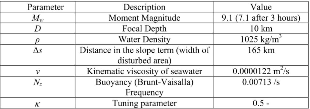
the water depths at 93 º E minus the water depths at 91.5 º E divided by 3∆s, where ∆s is the model grid distance. As depth changes horizontally, the slope changes along the source latitude, e.g. 2-11ºN. The source parameters for the present tsunami model are summarized in
Table 1. The time interval for numerical integration was 30 seconds to maintain numerical stability with the explicit solution. The porosity factor p was initially assigned a value of 1.0. The wind speed factor was assigned a very weak uniform magnitude of 1 m/s (from 80º). Numerical integration was done up to 48 hours only. With the 122 x 92 grid points of the present computational domain (38º-100ºE, 20ºS-25.5ºN), this took about 2 minutes run time in a Pentium 4 (2.8 GHz) computer.
Parameter Description Value
Mw Moment Magnitude 9.1 (7.1 after 3 hours)
D Focal Depth 10 km
ρ Water Density 1025 kg/m3
∆s Distance in the slope term (width of disturbed area)
165 km
ν Kinematic viscosity of seawater 0.0000122 m2/s
Nz Buoyancy (Brunt-Vaisalla)
Frequency
0.00713 /s
κ Tuning parameter 0.5 -
Table 1. Source parameters for the proposed tsunami generation model.
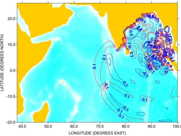
The results of the present modeling work are shown in a series of maps in Figures 4-8. Comparison of observed wave heights with the satellite altimeter data is shown in the time series graph of Figure 9. It can be seen in Figure 4 that the proposed generation model would produce a complex wave pattern of positive and negative values in the source region located near the ruptured fault line. The disturbed ocean water may not lie exactly above the ruptured fault. The assumption of a straight fault still showed a complex wave pattern due to the induced current oscillations from varying depths within the area. The computed wave heights after 1 hour showed a combination of positive and negative waves radiating away from the source region (Figure 5). Two hours after the quake, a distinct positive wave front shown by the red contours (flooding) has reached the eastern Sri Lankan coast (Figure 6). On the other hand, negative waves (drying) shown by the blue contours are predominant east of the source region. The formation of a series of waves can also be seen. Three hours later, the tsunami waves are shown by the model to suffer from refraction and diffraction in southern India (Figure 7). This is more pronounced 4 hours later as shown in Figure 8. The western side of Southern India is shown to be affected by the diffracted waves.
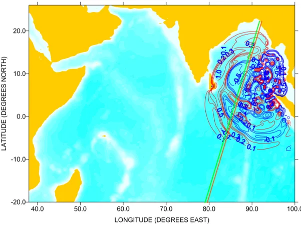
A comparison between observed and simulated tsunami wave height is shown in Figure 9. Due to the absence of numerical data, the altimeter data from the Satellite Jason-1 is shown along with the earlier computations of Pedersen et al. (2005). It is shown in the figure that a relatively good agreement between observed and modeled wave height occurs between 10ºS-10ºN. Using the proposed non-linear dispersive long wave model and the new generation mechanism, an improvement in model simulation can be seen between the Equator to about 5 ºN. The slight difference between observed and calculated wave heights after 10ºN could be the result of a combination of factors, both numerical and physical, such as the actual location of disturbed oceanic region, numerical dispersion due to large grid distance used, and early shoaling of the tsunami wave due to low spatial resolution. However, as the main energy lobe of the tsunami is concentrated at about 10ºS-10ºN, it is therefore important to have an accurate numerical simulation within this region which was demonstrated by the present model. Accurate model prediction especially with regards to wave amplitudes and phases can imply an improved warning system in terms of tsunami magnitude and arrival time.
40.0 50.0 60.0 70.0 80.0 90.0 100.0
LONGITUDE (DEGREES EAST) -20.0
-10.0 0.0 10.0 20.0
LAT
ITU
D
E
(D
EG
REE
S
NORT
H
)
Figure 4. Simulated wave height (m) 15 minutes after the earthquake. Red contour denotes positive wave and blue contour denotes negative wave.
40.0 50.0 60.0 70.0 80.0 90.0 100.0
LONGITUDE (DEGREES EAST) -20.0
-10.0 0.0 10.0 20.0
LA
TIT
UDE (D
EG
RE
ES
N
O
RTH
)
Figure 5. Simulated wave height (m) 1 hour after the earthquake. Red contour denotes positive wave and blue contour denotes negative wave.
40.0 50.0 60.0 70.0 80.0 90.0 100.0
LONGITUDE (DEGREES EAST) -20.0
-10.0 0.0 10.0 20.0
L
ATIT
UDE (
DEG
RE
ES
NO
R
T
H
)
Figure 6. Simulated wave height (m) 2 hours after the earthquake. Red contour denotes positive wave and blue contour denotes negative wave.
40.0 50.0 60.0 70.0 80.0 90.0 100.0
LONGITUDE (DEGREES EAST) -20.0
-10.0 0.0 10.0 20.0
L
ATIT
UDE (
DEG
RE
ES
NO
R
T
H
)
40.0 50.0 60.0 70.0 80.0 90.0 100.0
LONGITUDE (DEGREES EAST) -20.0
-10.0 0.0 10.0 20.0
LA
TIT
UDE (D
EG
RE
ES
N
O
RTH
)
Figure 8. Simulated wave height (m) 4 hours after the earthquake. Red contour denotes positive wave and blue contour denotes negative wave.
Figure 9. Comparison of computed and observed wave heights. The satellite data (Jason-1) were taken about 2 hours after the quake. The results of the present study are shown in green and orange lines along tracks shown in Figure 6. The blue line is from Pedersen et al (2005).
5.0 CONCLUSIONS AND RECOMMENDATIONS
It is shown in the present study that with the proposed generation model and dispersive wave model, the observed features of the Asian tsunami such as the initial drying of areas east of the source region, the initial flooding of western coasts, and the formation of a series of waves are correctly simulated. The new dynamic model for tsunami generation can be used to analyze the effects of various factors in the tsunami inception such as earthquake moment magnitude, fault-line orientation, focal depth of the earthquake, and various ocean properties
such as vertical stability and variable depths (e.g. bathymetric slope). The proposed tsunami propagation and transformation model can account for most of the observed wave characteristics as they travel through variable ocean bathymetry and coastal geometry. With adjusted parameter values, the tsunami model can explain the independent and combined effects of various factors related to the seismic disturbance and ocean properties where tsunamis occur. The new generation model may also be used to explain the occurrence of a series of large waves induced by landslides, volcanic eruption, or avalanches plunging in deep lakes or seas via the horizontal current acceleration that is produced. As long as there is a sufficiently strong horizontal current induced by such geological disturbances in a deep water basin, a series of waves can be created and modeled using the present model.
Model calibration requires accurate information about the earthquake magnitude, orientation of ruptured fault line, current amplitudes generated during the earthquake, accurate wave height observations and realistic frictional resistance coefficient. As observations of currents in deep waters during a tsunami are virtually absent, the present tsunami generation model has a major technological consequence as current meters are normally intended for deployment in shallow waters. Instead of measuring only the pressure at the seabed, deep-sea currents should be measured as well.
Another remarkable observation of the present study that merits careful experimentation is that tsunami inundation defies a classical oceanographic and hydrodynamic principle where wave breaking normally occurs whenever the wave height attains a certain fraction of the water depth. Due to its very long wave length, the wave breaking limit (i.e. maximum ratio of wave height to water depth previously believed to be about 1.2) may be far exceeded and tsunami waves do not readily break during propagation to shallow coastal waters. The hypothesis of a much higher breaking index awaits careful experimental study. In addition, the new generation mechanism may also be tested experimentally in a hydraulic laboratory. This requires accurate measurements of currents and waves which should be compared to the strength of the disturbing force.
Finally, the inherent complexity of tsunami generation and propagation in a complex ocean environment can always hamper a sensible tsunami warning system. But as new knowledge and understanding from accurately collected data and interpretation becomes available, these should be used so that a better warning system may be put in place. Accurate model prediction especially with regards to wave amplitudes and phases can imply an improved warning system in terms of tsunami magnitude and arrival time. To have a better simulation result, higher spatial resolution is needed and it is therefore recommended to have a grid distance as low as 1 min (as in Kowalik et al. 2005). The inundation of low-lying areas can be handled by using the wave output of such high-resolution model as input into a very fine mesh (50-250 m) within the devastated areas. Hazard mapping in populated coastal areas prone to floods from tsunami (or storm surges) definitely needs an ultra-high resolution in space.
REFERENCES
Abbott MB, McCowan AD & Warren IR (1984). Accuracy of short-wave numerical models. J. Hydr. Eng. Vol. 100, No. 10. pp. 1287-1301.
Dotsenko SF & Soloviev SL (1988). Mathematical simulation of tsunami excitation by dislocations of ocean bottom. Sci. Tsunami Hazards. Vol. 6, No. 1. pp. 31-36.
Koutitas C & Laskaratos A (1988). Tsunami-induced oscillations in Corinthos Bay: Measurements and 1-D vs 2-D Mathematical Models. Sci. Tsunami Hazards. Vol. 6, No. 1.pp 51-56.
Kowalik Z, Knight W, Logan T, & Whitmore, P (2005). Numerical modeling of the global tsunami: Indonesian Tsunami of 26 December 2004. Sci Tsunami. Hazards, Vol. 23, No. 1 p. 40.
Kowalik, Z (2003). Basic relations between tsunami calculation and their physics – II, Sci. Tsunami Hazards, Vol. 21, No. 3, 154-173.
Kulikov (2005). The highly dispersive waves of the Indian Ocean Tsunami. Russian Academy of Sciences.
Hunt, B. (1993). A mechanism for tsunami generation. J. of Hydraulic Research. IAHR. Vol. 31. pp. 111-120
Madsen, PA & Sorensen, OR (1992). A new form of the Boussinesq Equations with improved linear dispersion characteristics, Part 2: A slowly-varying bathymetry. Coastal Engineering. Vol. 18, No. 1, pp 183-204.
Merrifield M, et al. (2005). Tide gauge observations of the Indian Ocean Tsunami, December 26, 2004.
Nosov MA & Skachko N (2001). Non-linear mechanism of tsunami generation by bottom oscillations. ITS 2001. PMEL-NOAA.
Ortiz M, Gomez-Reyes E & Velez-Munoz HS (1999). A fast preliminary estimation model for transoceanic tsunami propagation. International Tsunami Symposium. 2001.
Pedersen, NH, Rasch PS, & Sato, T (2005). Modelling of the Asian Tsunami off the Coast of Northern Sumatra. Danish Hydraulic Institute Technical Paper. March 2005.
Peregrine DH (1967). Long waves on a beach. J. Fluid. Mech. 27, pp. 815-827.
Rivera PC (1997). Hydrodynamics, sediment transport and light extinction off Cape Bolinao, Philippines. 244 p. Balkema Press, The Netherlands.
Stelling GS (1984). On the construction of computational methods for shallow water flow problems. Rijkwaterstaat comms. No. 35, The Hague, The Netherlands.
Titov V, Gonzalez F, Mofjeld H & Venturato A (2003). NOAA TIME Seattle Tsunami Mapping Project: Procedures, Data Sources and Products. PMEL/NOAA. NOAA Technical Memorandum. OAR/PMEL -124.
Todorovska M & Trifunac M (2000). Generation of tsunamis by a slowly spreading uplift of the sea floor. Soil Dyn. Earth. Eng. Vol. 21, pp 151-167.
Villenueve, M & Savage, S. (1993). Nonlinear, dispersive, shallow-water waves developed by a moving bed. J. Hydr. Res. J. Hydr. Res. Vol. 31, pp. 249-265.
Wu, T Y. (1981). Long waves in ocean and coastal waters. J Eng. Mech. Div. ASCE. 107, No. EM3, pp.501-522.