Cette thèse porte sur l'étude de certaines questions liées à l'identifiabilité et à l'identification d'un problème de source inverse non linéaire. Cette thèse porte sur l'étude d'un problème de source inverse non linéaire qui consiste à l'identification de sources dans des équations de type advection-dispersion-réaction également appelées équations de transport.
Principales sources de pollution des eaux de surface
En effet, l'introduction de matière organique dans l'eau d'une rivière, par exemple, encourage les micro-organismes vivant dans cette rivière à participer au processus d'auto-épuration naturelle, c'est-à-dire qu'identifier les sources de pollution d'une rivière permettrait non seulement d'améliorer qualité de la vie humaine autour du fleuve, mais aussi préserver la diversité du milieu aquatique en apportant des réponses adaptées aux pollutions identifiées.
Conséquences de la pollution des eaux de surface
La pollution industrielle provient de tous les rejets industriels dans la nature sous forme d'aérosols (fumées ou poussières), dans les eaux usées et/ou les déchets industriels naturels. La dégradation biologique de certains déchets et le dépôt d'aérosols entraînent une pollution chimique et/ou organique des eaux superficielles et souterraines.
Indices renseignant sur la présence d’une pollution
Les nitrates constituent la dernière étape de l'oxydation de l'azote selon les réactions suivantes. L'approvisionnement provient principalement du lessivage des engrais artificiels et de l'azote reminéralisé sur les superficies cultivées, ainsi que des eaux usées et parfois des industries.
Modèle simple [DBO]
La somme de ces deux phénomènes détermine ce qu'on appelle le tenseur de dispersion hydrodynamique. Ici, kVk2 = qV12+V22 et DT, DL déterminent les coefficients de dispersion transversale et longitudinale tels que 0≤DT < DL.
Modèle couplé [DBO] − [OD]
In section 3, we demonstrate the recognizability of the source by measuring the BOD concentration at two observation points that frame the source area. In this section, we also prove that the features defining the searched source cannot be identified if the two observation points do not frame the source region.
Step1 : Localization of the source position S
In this section, we focus on creating an identification method that uses the data (III.9) to determine the elements defining the source F shown in (III.10). Let u be the solution to (III.4)-(III.7) with the time-dependent point source F presented in (III.10). To determine the two integrals in (III.39) involving the unknown data u(., T0), we prove the following proposition.
Proposition 4.3 Assuming that (III.11) holds, let T0 ∈(T∗, T)and µn0 be the eventual zero eigenvalue of the regular Sturm-Liouville problem presented in (III.12). Moreover, to determine the coefficients N ξn for n= 1, ., N by defining the truncated series in (III.42), we use the following system satisfied by u. This transforms the regular Sturm-Liouville problem introduced in (III.12) into the following equivalent normal Liouville form.
Note that, in view of the regularity of the coefficients D and v mentioned earlier in this article, the function h introduced in (III.50) belongs to L2(0, I).
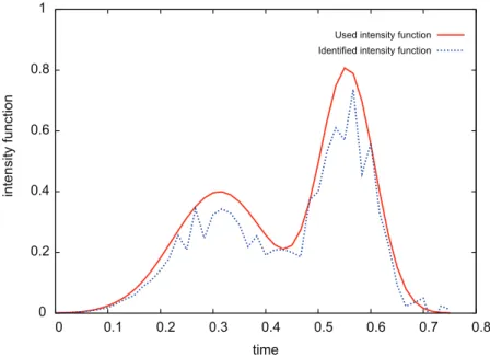
Step2 : Recovery of the time-dependent intensity function λ
In the remainder of this section, we focus on using (III.52) to recover the time-dependent intensity function λ. Since transport is naturally downward directed, it seems more convenient to use upward db concentration records than upward da records to identify λ. Therefore, according to (III.55), we only need to show that for all N ≥2 the two successive eigenfunctions ψN+1 and ψN+2 have no common zero in (0, l).
Otherwise we get a contradiction between the two signs on the left and right side in (III.62). Furthermore, using the same analysis, we prove that ζN+2 also has a zero located strictly between η= 0 and the first zero of ζN+1 and another zero strictly located between the last zero of ζN+1 and η=I . Since, in view of (III.3) and (III.48), there is a one-by-one correspondence between the zeros of the two functions ψn and ζn, then ψN+1 and ψN+2 have no common zero in (0, l ).
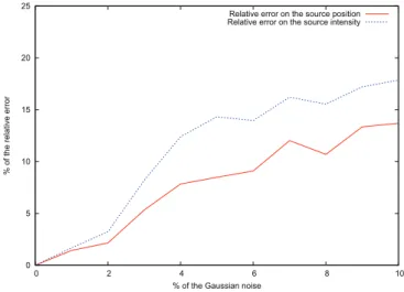
We end this section by analyzing the obtained numerical results and pointing out an outlook for the present study related to the Peclet number.
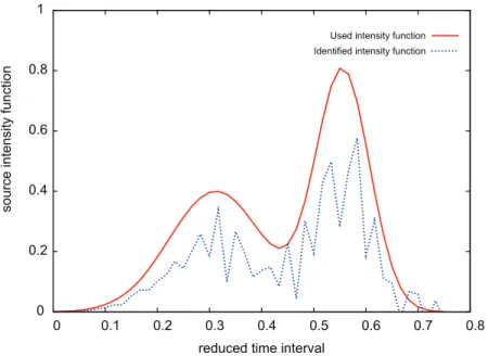
Undimensioned Problem
In addition, to calculate the N eigenpairs (µn,ζ˜n) for n = 1, ., N solutions for (III.66), we use the three-point finite difference scheme with the Numerov method [61].
Particular choice for the coefficients D, v and r
In addition, to determine the reduced source position ˜S from (III.75), we must prove the following result. To compute the diagonal matrix ˜H appearing in (III.68) using the function ˜h introduced in (III.67), we need to prove the following result expressing y as a function of the variable ˜η. Then, according to (III.48) and (III.79),˜ we derive the eigenfunction ˜ψn associated with the computed eigenpair (µn,ζ˜n) as follows.
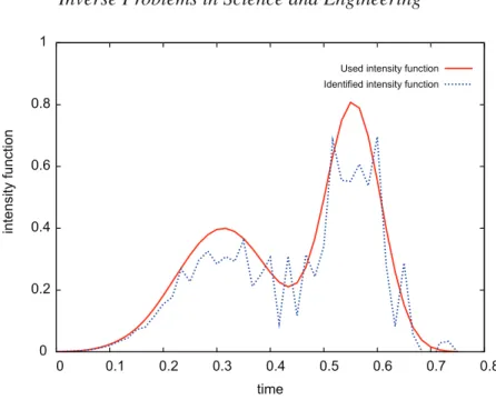
Numerical tests and discussion
L20, T;L2(Ω)∩C00, T;H−1(Ω) (IV.9) Furthermore, since the source position S is assumed to be an interior point of Ω, the condition u is sufficiently smooth on ∂Ω which lets then to define the boundary observation operator. For later use and as in the light of (IV.6) the matrix D is invertible in Ω, then there exists a unique vector fieldX solution of the linear system DX+V = 0 in Ω. Thus, using the results (IV.15) to substitute the associated terms in the right-hand side of the second equation in (IV.14), gives X=−D 1+D V .
From replacing the last expression on the right-hand side of (IV.27) with its value found in Then the boundary zero control problem presented in (IV.29)-(IV.30) is equivalent to finding γ ∈L2Γout ×(T0, T) such that the solution is Φ of the system. Then, by multiplying the first equation in (IV.43) by the solution in problem (IV.41) and integrating by parts over Ω using Green's formula, we obtain for allt ∈(0, T0).
It then appears from (IV.49) that the two source positions S(1) and S(2) solve the following system.
Localization of the sought source position
Source localization procedure
According to (IV.54)-(IV.55) and assuming that the coefficients P0, Pψ, Pψ⊥ obtained in (IV.55) are now fully known, we locate the sought source position S as the unique solution of the following non-linear system. We recall that the uniqueness of the solution S for the non-linear system (IV.61) is an immediate consequence of (IV.50)-(IV.51) from Theorem 3.1 Then, to determine the position S by using Newton's method, for example, we calculate the determinant det(Ja) of the 2×2 Jacobian matrix associated with the system (IV.61). Thus, using (IV.17) and (IV.19) one can use the following Newton's iterations to solve the system (IV.61): Given an initial guess x0 in Ω, calculate .
Computation of the HU M boundary control
For this purpose, we use the so-called inner product method [52], which is based on the use of the N × N matrix A as a representation of the linear controllability operator G∗G presented in (IV.67). Further, if kerek ∈L2(Ω) for all k≥1 then using the controllability operator introduced in (IV.67) and according to (IV.64) we obtain for all k, l≥1. Therefore, from (IV.69) and (IV.70) we obtain the results published in Proposition 4.4 ✷ Thus, according to (IV.67) and using the inner product method, we determine the minimizer ξˆ0 of the introduced functionalJ in (IV.34) from solving the following related linear system.
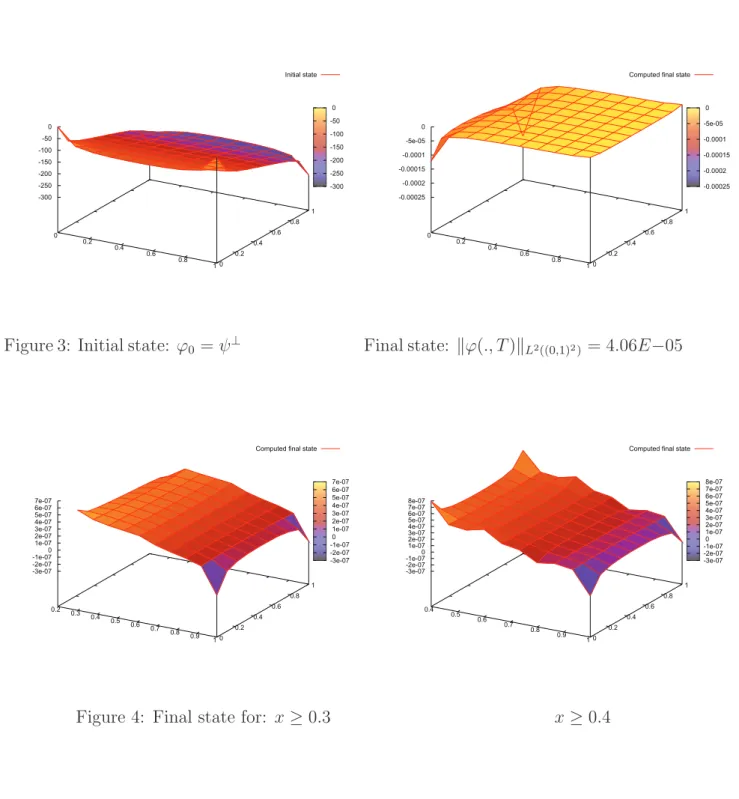
Due to the symmetry of the matrix A involved in the linear system (IV.71), it is only necessary to calculate half of its entries. Solving the linear system obtained in (IV.71) leads to the determination of HU M boundary control γ defined from (IV.35), which yields the boundary zero controllability problem introduced in (IV.29)-(IV.30) with a given initial state ϕ(., T0) = ϕ0 ∈ L2(Ω). D∇ek.νD∇el.νdΓ (IV.76) Since the minimizer of functionalJ is also approximated by ˆξ0 determined from solution of the linear system introduced in (IV.71), so that.
Therefore, an approximation of the HU M boundary check, defined in (IV.35) of Theorem 2.1, can be written as follows.
Identification of the time-dependent source intensity
Therefore, the identification of the unknown time-dependent intensity function λ(.) can be transformed to solve the deconvolution problem (IV.79). Therefore, using (IV.82), we derive a discrete version of the deconvolution problem obtained in (IV.79), which leads to the following recursive formula. As for the source position S = (Sx1, Sx2), we use the following approximation of the Dirac mass.
Thus, as established in the previous section, we locate the sought source position S as the unique solution of the nonlinear system introduced in (IV.54). To overcome this difficulty, authors generally assume in the literature that a priori information is available about the form of the source sought: e.g. In addition, we introduce the following boundary-zero controllability problem, that is, for a given τ ∈ (0, T) and an initial state ϕ0 ∈ L2(Ω), determine a boundary control γ ∈L2Γout×(τ, T) that determines the solutionϕ of the system.
Then the limit zero controllability problem introduced in (V.20)-(V.21) is equivalent to finding a limit control γ ∈ L2Γout× (τ, T) that leads the solution Φ of the following system.

Application to some frequently encountered pollution sources
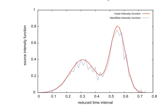
To that end, we need to determine the normalized eigenfunctions of the associated eigenvalue problem introduced in (V.27). In the remainder of this paper, we aim to evaluate the lower and upper frame bounds obtained in (V.48) from the total amount charged by the sourceF introduced in (V.51) for two different types of source intensity functions and various source positions. The numerical experiments in Tables 1-2 show that the constant value ζg=0(T0) achieved by the function ζg introduced in (V.43) with g = 0 yields good lower and upper frame bounds, as established in (V. .43). 48), which give a significant approximation of the total amount loaded by the time dependent point sources F in the case of one or more active point sources and for the two different types of source intensity functions used.
In this paper, we studied the identification of the time active limit associated with an unknown source appearing in the right-hand side of a 2D linear evolution advection-dispersion-reaction equation. We transform the determination of the sought HUM boundary control into the minimization of a continuous and strictly convex functional. We establish the calculation of the sought HUM boundary control for the general environment.
Lions, A Numerical Approach to Exact Boundary Controllability of the Wave Equation (I) Dirichlet Controls: A Description of Numerical Methods, Japan J. 2013) Identification of a Time-Active Boundary with Lower and Upper Bounds of the Total Quantity Imposed by an Unknown Source in the 2D Transport Equation, Inverse Problems and imaging submitted. Inverse Problems in Seismology, Bulletin of the Japan Society for Industrial and Applied Mathematics, Vol. 2003).