Long-Range (I)j

J.

Phj.s.

II France 6

(1996)

1759-1780 DECEMBER 1996, PAGE 1759

Theory of Long-Range Interactions in Polymer Systems

A-N- Semenov

(~'~'*)

(~)

Department

of

Applied Mathematics, University

of Leeds, Leeds LS2 9JT, U-K- (~)

Nesmeyanov

Institute of

Organo~Element Compounds

of Russian

Academy

of

Science,

28 Vavilova Str., Moscow l17812, Russia

(Received

15

July1996~

received in final form 12

August

1996,

accepted

2

September1996)

PACS.36.20.~r Macromolecules and

polymer

molecules PACS.68.45.~v Solid~fluid interfaces

Abstract. A mean-field theory of inhomogeneous polymer systems ^is

developed

in order to

include the finite molecular

weight

effects. A

general analytical expression

for the conformational free energy

providing

_a

bridge

between strong ^{and weak}

segregation

limits is derived. The

general

results _are further

employed

to obtain the

dependence

of interfacial tension in

polymer

blends

on the molecular

weights

of the components. ^A

long-range

repulsion

(induced by

the presence of

polymer ends)

between solid walls in

polymer

solutions and interfaces in

polymer

blends is predicted, the effect

being formally

due to finite molecular

weight

corrections. It is shown that this

repulsion

_can lead to _a stabilization of colloidal systems with small _amount of added

polymer

_even in the absence of _any specific interactions between polymer and particles. It is also shown that the end~induced repulsion _can lead to

freezing

of domain structures at late stages of demixing in polymer blends.

1. Introduction

Interfacial and surface

properties

of

multiphase polymer systems

are

important

both for _many

applications (such

_as

adhesion,

lubrication and stabilization of

colloids)

and for academic _rea~

sons. In

particular,

interfaces in

binary polymer

blends have been

intensively

studied both

experimentally [1-5]

and

theoretically [6-16]

for the

past

several decades. The

properties

of the interfaces _were discussed in terms of the

Flory

interaction parameter x, the number of links per chain N and other

geometric

characteristics of

polymer

chains. A mean~field the- ory of interfaces between immiscible

homopolymers (A

and

B)

in the

strong segregation limit, xN

_»

1,

was

proposed by

Helfand and co-workers

[7-9].

Their results for interfacial tension _~f and half-thickness A of an interface between

symmetric polymers (with geometrically

^identical

links)

_are

~f ⁼

~~)~x°.~,

^{zl =}

ax~°.~ (i)

where _a

=

b/@,

_{b is the} statistical segment of

polymer

chains, _v is the volume _per

link,

T the

temperature.

The

profile

of volume concentration of

A-links, #(z)

_e

#A(z),

is

#(z)

₌

p(z)

e 0.5

(1+

^tanh

(I)j (2)

(* ^e-mail: [email protected]

where _z

= 0

corresponds

to the interface

plane;

the

profile

for the B

component

is

#B(z)

=

1

d(z)

since the system ^is

incompressible.

The interfacial thickness in the

strong segregation

limit

(SSL)

is thus much smaller than the

typical

size of _a

polymer

chain: A _< R ₌

aN°.5,

which is

why

this limit is often called the

regime

of _narrow interfaces. Note that A _can be considered _{as an} effective correlation

length:

for distances _{z »} A the effect of the interface

exponentially decays

and becomes

negligible (see Eq. (2)).

Thus correlations due to

polymer

chain

connectivity, corresponding

to the scale

R,

are screened out

by

_monomer interactions.

(The

_same

screening

is known for _any concentrated

polymer system

^where the bulk correlation

length

is smaller than the chain size R

ii?].)

The

same

screening

is also

displayed by

_a

system

^of two

parallel

interfaces which

nearly

do not affect each other if the distance between

them, h,

is much

larger

than the correlation

length (see

Ref.

[18j):

the mean-field

theory predicts

that the interaction energy is

exponentially

small if h » £h

(in particular

the interaction is

negligible

for h

r~

R).

The last statements however _are

strictly

valid

only

in the limit of infinite molecular

weight,

N _{- cc.} Below _we show that the effect of chain ends

(which

_are

present

for _a finite

N)

results not

only

in _a renormalization of the interfacial tension

(and

other interfacial

properties)

but also

gives

rise to _an

important long-range

interaction between _any local

inhomogeneities

in concentrated

polymer systems.

In

particular

_we find that two

parallel

interfaces do interact _on the distances h

r~

R.

In the next

section,

_we

develop

_a

general

mean-field

theory taking

into account corrections to the free _energy due to

polymer

chain ends. From _a formal

point

of view the

theory

is _{an ex-}

tension of the

ground

state dominance

approach [17,19, 20]

to

systems

^which are characterized

by

_a continuous spectrum. ^The

general

results _are tested in the

regime

of weak

inhomogeneity

and _are then

applied

to

predict

the molecular

weight dependence

of the interfacial tension. In the fifth section the results _are further

applied

to treat interactions between

parallel

surfaces and also between small solid _or

liquid

inclusions in _a concentrated

polymer system.

^We show how the

predicted long

_range forces _may lead _{to a} stabilization of colloids

(emulsions)

with- out

adding

of _any

special stabilizing agents.

^The

problem

of interaction between interfaces in

polymer

blends is considered _as well. In the last section _we discuss another effect of the pre- dicted

long-range

interaction: _a

possible

termination of the domain

growth (effective freezing

of the domain coalescence

process)

_{at a} certain

stage during demixing

in blends of

incompatible polymers.

2. Free

Energy

of _a Finite Molecular

Weight Polymer System

This section is devoted _{to a mean} field consideration of

thermodynamic properties

of

a two-

component polymer

mixture

(a generalization

of the results to the _case of _any number of

components

^is

straightforward).

Note that the mean-field

approximation adopted

in this pa- per is valid if

v/b~

< 1

(see

Ref.

[20j

^for more

detail):

the corrections due to fluctuations

of the _monomer

density profile (not

considered

here)

_are

roughly proportional

to the small

parameter

u

/b~.

2.I. BACKGROUND. Let _us consider _a

system

^of two

homopolymers

A and B in _a

quasi-

equilibrium

state characterized

by

_some known

(given)

distributions of A and B monomers,

#A(r)

and

@B(r).

The

thermodynamic potential (effective

free

energy) corresponding

to this

state _can be

represented

_{as a sum} of three basic terms

accounting

^for the conformational

distributions of the

polymer

chains and monomer-monomer interactions

[20j

~ [lbA,

~Bj

_"

Finf

_{[lbAj +}

F$nf

_[lbBj +

tint (3)

N°12 THEORY OF LONG-RANGE INTERACTIONS IN POLYMER SYSTEMS 1761

where

F)~~

is due to a decrease of conformational

entropy (which

also includes translational

entropy)

of A-chains in the

inhomogeneous

state characterized

by

the distribution _PA

(r); F$~~

is the

analogous

conformational

free

_energy of B-chains. The last term

l§nt

₌

l~nt (IA, 48)

represents ^the free _energy of interactions between the _monomers. It is the term

l~nt

that determines the

compressibility

^{of the}

system

and also the

degree

of

incompatibility

of A and B links. The standard

Flory-Huggins

model

ii?]

_assumes that the blend is

incompressible

4A(r)

₊

iB(r)

" I

and also that the

density

of the interaction energy is

given by

a

quadratic

form of

#A

and _@B1

tint

"

~~~~ / lbA(r)@B(r)d~r (4)

U

where _u is the effective volume _{per one} link

[21j.

Although

the effects of finite

compressibility

and also

higher

order _terms in the

density

of the interaction energy

might

^be

important

in _{some cases}

[13j,

^the

Flory-Huggins

model

provides (at

least semi

quantitatively)

_an

adequate description

of most

polymer systems.

^In fact _many of the results

presented

in this paper are

actually

insensitive to the

particular

form of the interaction free _energy. We _use the

Flory-Huggins equation (4)

in all of the

examples

considered below in order to

keep

the

strongest

^{link with}

previous

theoretical studies.

The conformational free energy in the limit of

long

A chains

(NA

_-

cc)

is

[17,19,20j:

~2 (v j

)2

F)~~ [#A)

"

~

kBT

^~

d~r (5)

4U

#A

The contribution of B chains is

given by

an

analogous expression. Equation (5)

is valid if the characteristic scale of

inhomogeneity, I,

is much

larger

than the link size _aA

(the

continuous chain

limit),

and is much smaller than the Gaussian chain

size, RA

"

N(/~aA:

aA<I<RA

The conditions I » _aA, I » aB are assumed

throughout

this paper.

Note that for _a small

amplitude inhomogeneity, #A

=

(IA +6#A, b#A

_<

(#A), equation (5)

can be derived

using

random

phase approximation (RPA) ii?],

however this

equation

is valid

more

generally

for

arbitrary amplitude b#A.

Below

(to

the end of Sect.

2)

the conformational free _energy of the

A-component only

is considered. The size _a

= aA is chosen _{as a} unit

length,

and

kBT

_{as a} unit energy. We also omit index A in order to make notations

simpler.

Equation (5) implies

the so-called

ground

state

dominance;

it is exact in the limit of in-

finitely long chains,

N

=

NA

_{- cc}

(and

also for _a continuous model of

polymer chains).

A

generalization

of the

ground

state dominance

approach

for _a finite chain

system

is considered below. It is assumed that the chains _are still

long enough:

the coil size R is much

larger

than the

typical inhomogeneity

scale I

(say,

the thickness of interfacial _or surface

layer), aN~/~

» l.

For

simplicity

_we first consider _a one-dimensional

(d

=

I)

_{casej a}

generalization

of the results to

arbitrary

d is

straightforward

and is

performed

later. We calculate two correction terms to the dominant term,

equation (5),

which _are

formally proportional

to

1/,V

and

1/N~+~/~

Following

the lines first

proposed by

Lifshitz

[19j

we note that the conformational free energy

of,

_say,

A-component, Fcanf [4A),

is

actually equal

to the free _energy of _a

system

^{of A-chains} with _no excluded-volume interaction

(ideal system)

in _a

non-equilibrium

state characterized

by

a non-uniform concentration

profile, #(z

=

#A(z).

We will _assume first that _an

inhomogeneity

of the _monomer distribution is localized in the

region

_(z(

£ I,

_so that

p(z)

_-

do

in the

region

(z( » I. It is useful to consider the ideal

system

under external

field, U(z),

which induces the

given

non-uniform _monomer

density profile,

with

U(z)

_- 0 for _{z - cc}

[22j.

The conformational free _energy

(per

unit _area in _x, y

plane along

which the

system

is homo-

geneous)

is then

Fca~f [#j

= F

[Uj @Udz (6)

where

fl [Uj

= In

2

_{is the}

thermodynamic potential

of the

system

under the external field U As the chains do not

interact,

the

partition

function is

2

=

Zf IN!,

where

Zi

=

Zi [Uj

^{is the}

single-chain partition

function and

M

=

/ d(z)dz (7)

NV

is the total number of chains. Thus in order to find

Fcanf

_we need to calculated U and

fl [Uj.

The rest of the section is devoted to this task.

2.2. CORRELATION FUNCTIONS _OF IDEAL POLYMER CHAINS. A conformation of _a

single

chain is characterized

by

coordinates of all _monomers,

R(s),

0 < _s <

N,

where _s is the

monomer

position along

the chain. The

corresponding single-chain

Hamiltonian is

[23j

H

[Rj

=

jm ff ((f)~

_{ds +}

f/

_U

(R(s))

_{ds. The} statistical

weight

of _a chain with

given

end

positions,

z and z'

(the

Green

function)

is:

G(N,

_z,

z')

=

j

exp

j-H jRi) biz R(0))b(z' R(N))

D

jRi

The Green function

obeys

the

following equation [20, 24j

with the initial condition

G(0,

_z,

z')

=

b(z z').

The

general

solution of

equation (8)

_can be written in the form

G(N,

_z,

z')

=

~j ~fim(z)~i$(z')e~~'"

^~

(9)

m

where

~fim(z)

^and

Em

_are the

eigenfunctions

and

eigenvalues

of the

equation -~lclz)

₊

Ulz)~mlz)

₌

Em~l'mlz).

Equation (9) implies

summation _over all

eigenstates.

Below _{we are} interested in the _case of continuous rather than discrete spectrum. ^Moreover

we will _assume that the spectrum ^does not contain _any discrete branch at all. This

assumption

is validated in Section 2.3. In this _case two

eigenfunctions ~k(z)

and

~l-k(z) correspond

to each E

= k~

(note

that the lower

boundary

of the continuous

spectrum

is E

=

U(oo)

=

0):

~l'+ (U k~) ~k

= 0

(10)

Since the

complex-conjugated

function

~((z)

also must be _a solution of the _same

equation,

we can

always

choose

eigenfunctions

_so that

~l-~(z)

=

~li(z) iii)

N°12 THEORY OF LONG-RANGE INTERACTIONS IN POLYMER SYSTEMS 1763

Accordingly

_we rewrite

equation (9) keeping separately

the term

corresponding

to the

ground state,

^E = 0:

~~~'~'~'~ j~~~i~~~~

~

/_~ ~~~~~~~~~~'~~

_~~~

~~~~

The

eigenfunctions obey

the

following

normalization condition

/ ~l~(z)~li>(z)dz

=

2ii(k k') (13)

Note that

equation (10)

for k

= 0

implies

that

~o(z)

is

nearly

constant in the

region

_{)z) »} I.

We also _assume that

~o loo)

=

~fio(-oo) (see

Sect.

2.3).

It is convenient to normalize

~o

with the

following

condition:

~§o

(oo)

= 1. Below in Section 2.3 _we show that the function

~,o(z)

then becomes _a continuation of the

family ~§k(z)

in the limit k

- 0. The

point

^k ₌ o is excluded from

integration

in the second term in the r-h-s- of

equation (12).

The _reason

why

the E

= 0

term is treated

separately

in

equation (12) (in spite

of the fact that this term is

vanishing

in the

macroscopic limit,

V

-

oo)

is considered below.

Integrating

the function

G(N,

_z,

z')

_over the second coordinate _we find the statistical

weight

of _an N-chain with _a

given position

of _one end

only:

Wh~~~

v =

/ ~((z)dz

~~~~

is

nearly

the total volume

(length)

of the

system (as il,o(oo)

₌

1)

^and we define

Co

₌

f~o (I ~o) de, Ck

"

fi'((z)dz

for k

#

0. Note that both

Co

and

Ck

remains finite _in

the limit V _{- oo.} Note also that both definitions _are

actually

consistent since the scalar

product

of two different

eigenfunctions

must be _zero:

J ~§o(z)~§((z)dz

₌

0,

^k

#

0. Therefore

we can

generally

write:

Ck

"

/ ~((Z)11 #0(Z))

_dZ

(16)

We notice now that the first _{term for}

G(N,z) (corresponding

to E

=

0)

is not

vanishingly

small relative to the second _one: the E

= 0 term

gains

additional factor I'

during integration

over z'. That is

why

this term must be treated

separately.

The

single-chain partition

function is

Zi

"

f G(N, z)dz; using equation (14)

_we thus

get

Zi

" V

(1+ ~°

⁺

/

^~~

)Ck)~ e~~~~ (17)

1'

~

2K

Let _{us now} calculate the

profile

for the overall _monomer volume

concentration, #(z).

The

probability

to find the n-th link of _a

polymer

chain _at

point

z is

pn(z)

=

Zi In, z)/Zi>

where

Zi In, z)

is the statistical

weight

of _a chain with fixed n-th link. Two chain parts

(0, n)

and

(n, N)

_can be considered

independently (as they

do not

interact)

_as subchains of _n and N _n

links,

_one end of each subchain

being

fixed at

point

z. Therefore

Zi In, z)

=

Gin, z)G(N

_n,

z).

Summing

_over all _monomers of all

fit independent

chains _we obtain

#(z)

=

NV J pn(z)dn.

Taking

into account that

ufif/Zi

=

#o IN

in the

macroscopic

limit

II'

-

oo)

_we

finally get

the overall _monomer concentration:

#(z)

=

~° dnG(n, z)G(N

_n,

z) j18)

N

~

Note that in the limit N

- oo

(in

the

ground

state

dominance)

the second term in

equation (14) vanishes,

_so that

G(N

_-

oo,z)

=

~§o(z)

for V _{- oo} and therefore

#(z)

=

#oi'((z)

which is

a result of the

ground

state

theory [25].

However for _a finite N the second term

presents

a

correction:

G(N, z)

=

~§o(z)

+

b~§(z).

^In order to estimate this correction _we note that the

corresponding integral (see Eq. (14)

is

exponentially

cut off for k _> ko _"

N~~/~,

_{and also that}

in the

region

k

£

ko ^the

amplitude Ck

is of order I

(which

is the

typical

_range of

integration

in

Eq. (16) ).

^Therefore

b~l(z) ~ ~(

~

for _z

~ N~/~ Using equation (18)

we thus

get:

~~~~

~°~~(~~

~ ~

jl12

where the correction term is small since I _< R

=

N~/~

2.3. CALCULATION OF END-CORRECTIONS. In order to calculate

Fconf [#], equation (6),

we first need to find the external field

U(z)

which induces

exactly

the

given

_monomer

profile

when it is

applied

to the ideal

system

of

polymer

chains.

Obviously

this is _a

complicated

task

as itself. It is therefore convenient to

perform

the calculation in _a

slightly

different _way. We first find the field

Uo(z)

defined in the

following

_way: the _monomer

density profile

calculated for U

= Uo ⁱⁿ the

ground

state

approximation

must

exactly

coincide with the

given

distribution

#(z).

Then _we calculate the free _energy of the

system

under the field Uo ^{and find} correction

iii (z)

to the _monomer concentration

profile

_on the

top

^{of the}

ground

state

approximation.

After that the

corresponding

correction to the field 6U

=

WI

needed to compensate ^for

b#i

will be determined.

Finally

the correction to the free energy related to

[Vi

is calculated

(~).

According

to the definitions above the

ground

state

eigenfunction, ilo(z), corresponding

to the field

Uo(z),

is

strictly

related to the

given density profile:

~Yiiz)

=

) jig)

so that in

particular

~Yol-cxJ)

₌

lYo(co)

₌ 1

Using equation (10)

_~n.e thus

get

q/,,( ~2

~°~~~

_"

v)())

"

'~°'~~~~WI~°~~~~

^~~°~

Note that the field Uo defined in

equation (20)

does not

produce

_any discrete spectrum

(with

E _<

0)

since

ilo(z)

is real and

positive everywhere

and therefore must

correspond

to the

ground

state.

Let

I

_{[U] be the exact}

equilibrium

_monomer

density profile

induced

by

the field U:

#

[U] =

if [U] /bU,

where

fl [U]

_is defined after

equation (6).

In

particular #

_[Uo]

=

#+ iii

where

#(z)

is the

given density profile

and

iii

is _a small correction _to the

ground

state result.

Adding

_a

correction W to the field _we write

(in

the linear

approximation) #

_{[Uo +}

ll'j

cf

#

₊

b#i l/l§",

where

l/

_is

a linear operator,

I/H~(z)

_e

J I[(z, z')W(z')dz'.

Therefore the external field _we

are

looking for,

U

= Uo +

WI,

is

specified

in the main

approximation by

the

equation

l/l§1

=

h#1 (21)

(~) ^The same

general

strategy _was

adopted

in reference [16].

N°12 THEORY OF LONG-RANGE INTERACTIONSIN POLYMER SYSTEMS 1765

Let _us define the free _energy functional F

[U, ii

=

fl [U] J U#dz,

where both U and

#

are

formally

treated

independently.

The conformational free _energy

(Eq. (6))

is thus

indirectly

defined

by equations Fconf [#j

= F

(U, I [U]j, #

[LTj =

#. Using general

relation bF [U,

#j

~~ ^"

# (U) #

and the relations above _we find that

~~

~~)/j ~'~~

^cf

-k (W lf~i

in the main

approximation. Integrating

back the functional derivative _we

get

Wilz)

F~~nf iii

₌ ^F _[Uo +

lf'i, II

=

Fo

+

/

dz

/ dIV(z)

_K

(WI W)

=

Fo

+

Fi (22)

o

where

Fo

₊ F

[Uo, II

and

~ / ~~~~~~~~~~~~

_~~~~

Below _we show that

Fi

is

typically proportional

to

1/N~/~ (for

one-dimensional

case).

There- fore _we need to calculate this term in the main

approximation only

since

higher-order (in 1IN)

corrections _are

neglected

here.

Using equations (17, 7, 15, 20)

_we

get

Fo

= F* ₊

~

dz ~

(li 4)

_d=

~°

^~~

)Ck)~ e~~~~ (24)

4u

/

NV

/

NV

/2K

where _we take into account that

V#o

"

fifNv (see Eq. (19)) [26].

Here F*

=

fifIn )

is the

ideal-gas

free energy of the

corresponding homogeneous

_sys-

tem. The second term

(which

is

exactly equal

to

J Uo4dz)

is the well-known

output

of the

ground

state

approximation (compare

with

Eq. (5)).

The last two terms represent ^{the finite} N corrections which _are

proportional

to

1IN

and

ko IN

mJ

1/N~/~ correspondingly.

Let _us turn to calculation of the last correction,

Fi Using equations (14, 18)

_we find in the main

approximation (and

in the limit V _-

oo):

~~~

_{~~~ "}

j~

lYo(z) /~

_d~

/

^dk _~ ~~

° ~~ ^~~

~~k(~)

_~~

where the functions

ilk (z)

_are defined in

equation (lo)

with U

=

Uo,

and

ilo(z)

is defined in

equation (19).

We _now have to find the functions

4fk(z).

Note that since

typical

n r~ A~ in the r-h-s- of

equation (25),

_we

only

need to consider small

enough

k

~

ko =

1/N~/~:

the

integral

is cut-off for

larger

wave-numbers.

Taking

into account

equation (20)

^{and the fact that}

ilo(z (Eq. (19)

tends to

unity

in the

region

_)z) »

I,

_we conclude that

Uo(z)

vanishes in this

region (in

the most

interesting

_cases the decrease of

Uo(z)

is

exponential).

It is useful to

split

the

problem

and consider first the behavior of the functions

ilk(z)

in the outside

region

_)z) » I. Here

equation (lo)

reduces to

il[(z)

₊

k~ilk(z)

" 0

implying

a

general

solution in the form:

ilk(z)

= Ae~~~ ₊

A'e~~~~,

z <

0; ilk(z)

=

Be~~~

₊

B'e~~~",

_{= >} 0.

Obviously

A and A' _must be linear combinations of B and B':

Here _we take into account that both

ilk(z)

and

il((z)

_are solutions of

equation (10).

We thus define _a

family

of solutions of

equation (10)

^which

additionally debend

_on two free

parameters

B and B'.

Taking

into account that substitutions k _-

-k,

B _-

B',

^B' _-

B,

A _-

A',

A'

- A

together

does not

change

the

eigenfunction

at all, _we

get

the

following general

relations:

a(-k)

=

a*(k), fl(-k)

=

fl*(k) (2i)

Another

general property

of the functions _a and

fl

follows from _energy conservation

[27j (within analogy

of

Eq. (10)

and

Schr6dinger equation):

lal~

₌ I +

lfll~ 128)

Let _us

form611y

set B

=

1,

B'

=

0,

^{and consider the} limit k

- 0; the _z > 0

asymptotics

is then

ilk(z)

= e~~~ _- 1.

Obviously equation (10)

with U

= Uo

(Eq. (20)) implies

the

only

solution with this

asymptotics, namely

the function

ilo(z) (Eq. (19) ).

Therefore

limk-o ilk (z)

and

ilo(z)

_must coincide also in the

region

_z <

0,

_{)z) »}

I,

where

ilo(z)

_-

1,

_so that

a(o)

₊

fl*(o)

=

(2g)

Now

using equations (27-29)

_we obtain

a(0)

₌

1, fl(0)

= 0. Both

o(k)

and

fl(k)

must be

regular functions;

their

expected

behavior for small k is:

a(k)

₌ 1+

iO(k), fl(k)

=

O(ik).

As the

only

characteristic scale in the

eigenvalue problem (Eq. (10)

is

I,

we can rewrite the above

relations _as

o(k)

= 1+

iO(lk), fl(k)

=

iO(lk) (30)

In the relevant

region

k

~

ko ^the corrections _are of order

lko

"

I/N~/~

_<

1,

_{and thus}

can be

neglected

in the main

approximation.

The actual values of the

parameters

^{B and B'} must be chosen in order to

comply

with the normalization conditions

(Eq. (13))

which

imply

the

following

relations:

AA'+ BB'

=

0;

_)A)~ +

)B')~

₌ 1

(31)

Equations (31. 26) completely

define the

A, A', B,

B' _{up to a common}

phase

which _can be fixed

by assuming

that B is _a

positive

real.

(We

also _assume that )B~) <

)B).) Using

also

equations (30)

_we thus

get

^A ₌ 1+

iO(lk),

B

= 1+

O(l~k~),

A'

=

iO(lk),

B'

=

iO(lk).

Omitting

corrections of order

I/N~/~

we thus obtain

ilk(z)

_cf e~~~ for )z) » I. Therefore in the limit k _- 0 the function

ilk (z)

coincides with

ilo(z)

_as claimed above

(since

both functions

reveal the _same

asymptotic

behavior and

obey

the _same

Eq. (10) ).

It is _easy to check _now that inside the

inhomogeneity region,

_)z)

mJ

I, ilk (z)

coincides with

ilo(z) again

within _{an error} of order lk. Therefore in the main

approximation

we

get

the relation

ilk(z)

_cf

ilo(z)e~~~ (32)

which is valid

everywhere

_up to a correction

mJ lk which is small

provided

that k

£ ko.

With

equation (32)

the correction

iii (Eq. (25))

_can be rewritten _as

Substituting equation (32)

into

equation (16)

_we

get

Ck

"

/ ilo(z)

II ilo(z)) e~~~~dz (34)

N°12 THEORY OF LONG~RANGE INTERACTIONSIN POLYMER SYSTEMS 1767

We _{are now} in _a

position

to find the

operator l/. According

to its definition

(see Eq. (21)

and

above)

the

corresponding

kernel is

Kjz, z')

i

jji~)~

where

#

₌

I[Uj

is the _monomer distribution

corresponding

to the field

LT(z).

The fluctuation theorem

[28j

^then ensures that

h'(z, =')

is also

equal

to the correlation function of _monomer

density

for the ideal

system

under the field

U(z): K(z, z')

=

(#(z)#(z')) (#(z)) (#(z')),

where

mean the

thermodynamic

_average.

Taking

into account that the chains do not interact _we thus

represent

the kernel _as

fif~2 K(z, z')

=

/ dndn'G(n, z)G(n', z')G(N

_n

n',

z,

z') (35)

21

where three factors in the

integrand

constitute the statistical

weight

of _a

polymer

chain with n~th link fixed at

point

_z, and

(N n')-th

link at

point

z'. In the main

approximation

_we

keep only

the first term in the r-h-s- of

equation (14): G(n, z)

_m

ilo(z). Substituting equation (32)

into

equation (12)

and

neglecting

in the last

equation

the first term which vanishes in the

thermodynamic

limit, _we

get: G(n,

_z,

z')

_m

ilo(z)ilo(z') J fle~~l~~~')e~~~'~

^Thus we rewrite

equation (35)

_as

~~~'~'~ ~°~~~~~~~~~~~'~ / ~

~~~~~

~'~~~ ~~~~~

_~~~~

where

fD

is the

Debye

function

fD(it)

=

[(it

+ e~~

-1) 137)

Now

using equations (21, 23,

33,

36)

after _some transformations _we

get

~i

₌

) / j)

ic~12 (£ (1- -N~2jj

^{~ i}

fD(Nk2 (38)

Finally using equations (22, 24, 38)

we obtain

[29j

where

e~"(u

+

1) f(~)

~~~~

"

~ l + e-~

CL

"

/ Q(Z)e~~~~dz 141)

~(z)

₌

w@ <(Z)/<o (42)

As in

equation (24)

the first term here is the

ideal-gas

free _energy of _a

homogeneous system,

the last two terms

represent

corrections to the

ground

state

square-gradient

free _energy due

to finite

length

^N of

polymer

chains. Note that the corrections are

formally proportional

to

1/N

^and to

1/N~/~ correspondingly.

The dominant end-correction of order

1/N only

_was

previously

calculated in reference

[30j using

_a

slightly

different

approach

first

suggested

in

references

[31,32j.

The

present

^result

(Eq. (39)

is in

agreement

^with that obtained before

[30j.

An

analysis

shows that the result

(Eq. (39))

is valid within _{an error} which is

proportional

to

1/N~.

The small parameter

implied

is

actually Co/R,

where R

=

N~/~a

_{is the coil size,}

if the

inhomogeneity

of _monomer distribution is localized in the

region

of size R. The _con- dition

Co /R

< 1 in

particular implies

that either _an

amplitude

of the function

~(z)

is small

everywhere (max )~(z))

<

1,

^I-e-

)b#(z))

<

1,

^where

b#(z)

_e

d(z) #o),

_or the

inhomogene- ity

is

pronounced

but is localized within _a

region

which is much _{more narrow} than R. More

generally

_we can consider also _{a sequence} of

pronounced

local

inhomogeneities (of

width

I) separated by

distances much

longer

than I. The above results _are valid if

iii

_<

lo Using equations (33, 41)

we find that

iii flu

r~

4(z),

where

fi(z)

is

given by

the

integral

in the r-h-s- of

equation (33): fi(z)

₌

(~(z).

_{The operator}

(

_{here in the Fourier}

representation

is

S(k)

ill e~/~~~ );

this

operator

^therefore

performs smoothing

_{over a} scale _r~

aN°.5

=

= R. Thus

the most

general

condition of

validity

of

equation (39)

is that smoothed

~(z)

is small:

fi(z)

< 1.

Equation (39)

is the main basic result of this _paper. It is

interesting

to check the result for the _case

if

_weak

inhomogeneity, )b#(z))

<

1,

where the free _energy is known

exactly

_{[17] as an}

expansion

in

ii

=

# #o (up

to 2nd

order):

~°~~ ~~~

_{~ ~~~~}

/

~~~~~~~

~

~/v#o ~ fD

ji~a2k2

~~~~^~ ~~~~

where

b#k

is the Fourier

image

^of the function

6#(z), Fr~f

=

fi J #o

In

fidz

is the reference free _energy of the

homogeneous system

^with

#(z)

_e

#o,

and _pr~f

=

fiIn )

_{is the}

corre-

sponding

chemical

potential. Expanding

r-h-s- of

equation (39)

in

analogous

series up ^to the

quadratic

order _we

get

the result which

exactly

coincides with

equation (43)

_as it should be.

So far _we assumed that

#(z)

tends to

#o

in both limits _{z - oo} and _{z - -oo.} It is

possible

to

generalize

the basic result

(Eq. (39)

in order to include also the _case

#(z)

_-

#o

as z - oo,

#(z)

_- 0 _{as z}

- -oo

provided

that

#(z)

vanishes

rapidly enough

_on the scale I _< R. To

simplify

the

argumentation

let _{us assume} that

#(z)

_e 0 in the left-side

region

_z < _zw

[33].

Let _us shift the coordinate

origin setting

_{zw =} 0 and introduce _a

reflecting

wall to the left of the

system

at the

point

_zw. It is obvious that the wall would not

change

the free _energy of the

system

^{since the}

polymer

does not penetrate down to _zw anyway. The

reflecting

wall

boundary condition, fl

= 0 at _{z =}

0,

should be valid _not

only

for the total

density,

but also for all other

monomer distribution

functions,

in

particular

^for the

eigenfunctions

of

equation (10).

Let _us

now

complement

the _monomer distribution

#(z)

and the field

U(z) by

their mirror

images

in the

region

_z < 0 and then _remove the wall. Due to the mirror

symmetry

the _new

(extended)

system must be characterized

by

both _even and odd

eigenfunctions.

It is easy ^to check however that odd

eigenfunctions

does not contribute at all to the free _energy, whereas _{even ones}

just

coincide with the

eigenfunctions

for the

original system

in the

region

_z > o. Therefore the one-chain

partition

function

Zi

is the _same in both cases, and the total free _energy of the extended

system

is

exactly

twice the free _energy of the

original system.

Next _we note that the mirror extended

system

^does

obey

the _necessary condition:

#(z)

_-

#o

for _{z -} +oo.

Obviously

the mirror extension

implies

the

following

transformation of the

amplitudes: Ck

_-

Ck

₊

C-k Finally

_we calculate the free energy of the mirror extended

system using equation (39)

with the _new

amplitudes Cki dividing

the result

by

2 _we thus

get

N°12 THEORY OF LONG-RANGE INTERACTIONSIN POLYMER SYSTEMS 1769

the conformational free _energy of _a semi-infinite

system:

~2

(d#/dz)~

= ~~

/ #(~~

^~~

e~i'~~

^~

~~

~

~

(44)

~~~~ ~~

lo j°°

^~~

f(Na~k~ )Ck

+

~~~~

~C0

+

@

_~

2K

In order to

get

the conformational free _energy of _a

particular polymer component (say, l~(~~)

we need to

change N, #,

_a and

#o

to

NA, IA,

_aA and

#oA. Equations (3, 4)

and

(39)

or

(44)

thus define the free _energy of _a one-dimensional two-component

polymer system.

3. Molecular

Weight Dependence

of Interfacial Tension in

Binary Polymer

Blends

The results obtained in the

previous

section _are

applied

to _some

particular systems

^below.

As _a first

example

let _us consider _a blend of two

incompatible polymers NA, NB

in the

strong segregation limit, XNA

»

1, XNB

» 1. In this _case the

system separates

into two

macrophases:

almost pure A and almost pure

B; #A(z)

_e

#(z)

_-

I,

_{z - oo;}

#B IQ)

= I

#(z)

_-

1,

z - -oo.

For

simplicity

_{we assume} that A and B links _are

geometrically

similar: _aA

" aB " a.

The free energy of the

system

is defined

by equations (3, 4, 44).

Both

~A(z)

_e

fi@

#A(z) (note

that

#o

"

1)

and

~B(z)

vanish outside the interfacial

region

of width

r~ A. There- fore the

amplitudes Cl

and

Cf nearly

does not

depend

_on k in the relevant

(for Eqs. (39, 44) regime,

k

r~ ko "

1/R,

since

koA

< 1.

Omitting

the terms which _are

directly proportional

to

the number of chains

(like

F* in

Eq. (24))

_we thus write:

F = Fg~ +

F~nd (45)

where Fg~ ^{is the}

ground-state

free _energy

and

F~nd represents

the finite N corrections:

where

Cl

=

J (fi #) dz, Cl

=

J (@@

₊

#)

dz.

Minimization of the dominant _term Fg~ ^{leads to the well-known} characteristic _monomer

density profile d(z)

=

ji(z),

_where

j(z)

is defined

by equation (2).

The correction term,

F~nd,

induces _a

perturbation

of order

1IN (here

N

r~

NA

r~

NB).

However since

#(z) corresponds

to the minimum of

Fg~,

^the

corresponding change

_{of Fg~} is of order

1/N2.

Thus in order to

get

^the interfacial tension within _{an error} of

Oil /N~)

_we could

just

substitute

equation (2)

in

equations j45-47);

the result is:

~ = lo

i

2 in 2 _{+ +}

~

~~~ +

~

~~~

+ O

~

(48)

XNA iNB (RNA) (~NB) (XN)

where

~ ~

K

=

~~~~~

/ f(t~)dt

m 0.5921

K -co

and _~o

"

)x~/~

is the zero-order result

(see Eq. ii)).

In

particular

for the

symmetric

_case,

NA

"

NB

"

N,

the molecular

weight dependence

of the free _energy is

given by

~(N)

m j

~'@

+

'~~~~ l(49)

~

(XN)

This

equation

^is

asymptotically

exact in the limit

xN

» 1

(within

_{an error} of order

1/(xN)~).

However it

apparently provides

_a

good approximation

_even in the

region

where

xN

is not

large.

In

fact,

the

symmetric system

is

separated

if

xN

_> 2

[17];

^{at the critical}

point, xN

=

2,

the

tension must

vanish,

_~

= 0.

Substituting xN

= 2 in

equation (49)

_we

get

_{~ =}

0.03~o.

It thus

seems

likely

that the absolute _error of the

expression (Eq. (49))

is not

larger

than

3i~

of _~o

everywhere.

The first correction to the tension

(of

order

1/~N)

_was calculated

previously

in several papers

[11-13, 30j.

The numerical

prefactor

obtained in reference [30] agrees with that in

equation (49),

while other

approaches

lead to different

prefactors

due to some additional _ap-

proximations

involved

(see

Ref. [30] ^for more

discussion).

As the last comment here we note that the

molecular-weight dependence

of the interfacial

tension _comes

entirely

from the

N-dependence

of the conformational free _energy. This _con- clusion is in

disagreement

with _a statement of reference

[16]

^{it is claimed there that if the}

O(1IN)

correction to ~ is _nonzero, then it must be due to

molecular-weight dependence

of the interaction energy

(the

fact that the

~(N) dependence

_was considered in Ref.

[16]

^{at constant} pressure rather than constant total

density

does not make _any difference for _an

incompressible polymer system).

It _seems therefore that the

corresponding

statement of reference

[16]

can not be

general

if valid at all

[34].

4. Semidilute

Polymer

Solution _{near a} Wall

Here _we consider another

example

_a

homopolymer

solution _on the

right

to _a hard wall at z = 0. The solvent

quality

is assumed to be

marginal

_so that _a mean-field

theory

_can be

applied.

The bulk volume concentration is

#(oo)

=

#o.

The interaction free _energy in the second virial

approximation (which

is valid if

#o

is small

enough)

_can be written _as

l~nt

"

~ /#~(z)dz (50)

2u

Here

fl

is _a numerical factor

depending

on the solvent

quality.

Local

polymer-wall

interactions _can be adsorbed in _an effective

boundary

condition

lj ())

= a

lsi)

z=o

The wall is

repulsive

if _{o >} 0 and is

adsorbing (attractive)

if _a < 0. The Edwards bulk correlation

length (

₌

a/@$

is assumed to be much smaller than the coil

size,

R

=

aN~/~

Minimization of the free _energy

Fiji

=

l~nt

+

F~onf

defined

by equations (44,

50,

51)

leads to the

following equilibrium

total _monomer distribution:

4(z)

₌

#s(z)

₊

41(z)

where

~ ^z

(52)

Is (Z)

"

#o

ta°h

fi

^~

~°°~~

N°12 THEORY OF LONG-RANGE INTERACTIONS IN POLYMER SYSTEMS 1771

is _an

output

^of the

ground-state approximation (note

that const here

depends

_on

a).

The relevant

screening length

is

short, (

<

R; #~(z)

_cf

#o

in the

region

_z »

(.

The second term is

a

relatively

small but

long

_range correction which is molecular

weight dependent:

~~~~~

~° flj~~3/2

_~

j~

_~~~~

~~~~~

~it)

= 2

/ ()f(k~)

e~~~

and the reduced

amplitude Co

"

f(/$ Is flu )dz. Obviously Co

~

f.

The

typical decay

scale for

ii

is thus of order of the coil size

R,

and its

typical amplitude

is 11 ~

lo / (flN#o

_)~~~

The

long-range

effect of _a hard wall had been

previously

considered in references

[15,16j using

different

partly

heuristic

approaches. Fortunately

both the

previous

results and

equation (53) completely

_agrees with each other.

It is worth

noting

that for the _case of localized

inhomogeneity

the end-corrections to the

ground

state conformational free _energy

(last

two terms in

Eq. (39) depend

_{on a}

single integral

parameter, the

amplitude Co

"

f (fi~ 4/40)

_{dz. This is due to the}

following physical

reason which _was

originally

^formulated

(independently)

in references

[15j

^and

[16j

^and was then

used _{as a}

starting point

for the theoretical

approaches developed

in these papers.

Within the

ground-state approximation

the _monomer

density

is

directly

related _to the

ground-state eigenfunction: #(z)

=

#oi'((z).

Let _us mark _one end _per each chain. The distribution of the marked

points

is

c~(z)

₌

fifG(N,z)/Zi Using

now

equations (14, 17)

and

retaining only

the first

(ground-state)

terms in the r-h-s- of these

equations

we obtain

c~(z)

=

)~§o(z).

If _{we now} take into account that the volume _per chain is

NV,

the total

polymer

volume calculated from end-distribution would be

J

_polfio

(z)dz,

I.e. different from the

volume

coming

out from the total _monomer

concentration, J #(z)dz.

The

difference,

/[#oi'o(z) #oi'((z)jdz

_e

#oco (54)

is

just proportional

to

Co,

which is thus a measure of _a mismatch between two distributions.

For the _case of _say

repulsive

wall

(#(0)

=

0)

the difference is related to the fact that the

probability

to find _an end

point

_near the wall

(which

is

proportional

to

~§o(z))

^is

higher

than that for _a middle link

(proportional

to

~§((z)).

The mismatch

(Eq. (54)

indicates _an intrinsic

error inherent to the

ground

state

approximation.

Obviously

both end and total _monomer distributions _must be

slightly

^corrected on scales

larger

than

( (note

that _a small correction in the

region

_z

mJ

(

could not

possibly compensate

the

mismatch)

in order to make them consistent with each other. Since there is _no other

typical

scale

larger

than

( apart

from the coil size R it is

anticipated

that the corrections to the distributions _are universal functions of

z/R

with the

amplitude proportional

to the initial

mismatch,

I.e.

proportional

to

Co-

5.

Long-Range

Interaction in Concentrated

Polymer Systems

At the end of the

previous

section _we show that end-effects lead to a

long

_range

perturbation

of

polymer density

_{near a} hard wall. Below _we consider interaction between surfaces

and/or

interfaces caused

by

the same source.

5.I. INTERACTION BETWEEN Two PARALLEL SURFACES. Let _us consider two

parallel plates

immersed in _a semidilute solution

assuming repulsive polymer-wall

interaction

(a

_{- oo}

in

Eq. (51)).

For _a

single plate

the _monomer

density profile

in the

ground

state

approximation

is defined

by

the well-known law

Ii?] given by equation j52)

with const ₌ 0:

<(z)

-

<o tallll~ Ill (55)

where _z is the distance _to the

surface,

and

(

₌

a/@%.

Far

enough

from the surface

(z

»

()

the

perturbation

is

exponentially

small:

#(z)

_m

#o 1

4e~~/~j

In the _case of two

plates

at _{z =} 0 and _z

= h

perturbations

induced

by

each

plate

_are additive in the

region

_z »

(,

h _z »

(:

4(z)

_m

do 1 4e~~/~ 4e~lh-z)/fj

The force of interaction between the

plates (per

unit

area), predicted by

the

ground

state

theory, fgs,

is

directly

related to the concentration in the

middle,

at _{z =}

h/2 [35j: fgs

₌

) (#(h/2) #o)~.

_{The minus}

sign

means that the force is

always

attractive. Thus _we

get

fgs

₌

-32~#(e~~/~ (56)

u

Let _{us now} calculate the end-corrections _to the interaction force.

Unfortunately equation (39)

cannot be

directly applied

to the _case of

polymer

solution confined between two

plates

since

the

plates completely separate

^{the confined}

system

^from the outside solution. However it is

possible

to

generalize equation (39)

in order to include the confined _case

using

the idea which

was

already employed

to treat a semi-infinite

system (to

derive

Eq. (44) ).

^We

formally

consider the actual

planes

_as

being reflecting. Considering

^all

possible images

of the

original

confined

system

^{in these mirrors} we thus _come to _an

infinitely periodic (in

_z

direction) system,

with

periodicity

h. It is then _{easy to} show that the free _energy of the resultant infinite

system

_per

period

coincides with the free energy of the

original

_system. The free energy of the infinite

system

can be calculated

using equation (39).

The final result for the free _energy of the

original system

^is:

~°~~ ~~ Iv /

~~~~^~~

e~u

^{~~ ~}

~ / ~~~~~~

_~~

~~ ~°

~

4i~jiu ~j ~~~~~~~~

^{~~~ ~}

~~~~~

^~~~~

where the _wave number k

adopts

discrete

values,

km =

)n,

n ₌ 0,

+1, +2,..

It is the last term that determine the

long-range

interaction

(for

h _»

().

The

amplitudes Ck

_can be calculated

within the

ground-state approximation. Taking

into account the

symmetry

of the

system

(j(z)

₌

#(h z)),

_we

get Ck

_"

2C)~~

^{if k} = km with _{n even,} and

Ck

₌ 0 if k

= km with _n

odd,

^where _C)~~ ^{is the}

one-plate amplitude

defined

by equations (41, 42)

with

#(z)

defined

by equation (55).

^We can

neglect k-dependence

of C)~~ ^{since the} relevant wave-numbers _are

N°12 THEORY OF LONG-RANGE INTERACTIONS IN POLYMER SYSTEMS 1773

small,

k

r~

1/h

_<

1If,

where

(

is the

typical

localization scale

corresponding

to the function

~(z)

for _one

plate.

Thus _we find C)~~ ^m

Cj~~

=

2((1

In

2).

It is easy ^to show that the second and third terms in the r-h-s- of

equation (57) nearly

do _not

depend

_on

h,

_so that

h-dependence

of the free _energy is determined

by

the last term

although

this term is subdominant

according

to its absolute value

(the

first term

gives

rise to the trivial

ideal-gas

_pressure which is

exactly compensated by

similar pressure

acting

_on the

plates

from

outside). Omitting

constant terms in

equation (57)

_we

get

the

long-range

_energy of interaction

(per

unit

area)

where

n

0.61617, and +

~

T ~ T

is the

reduced

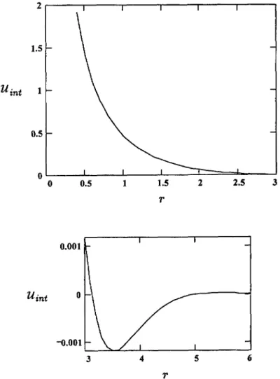
unction lotted in Figure 1.

In the

region h

» R

the

the haracteristic decay

length oforder

_[36j.

In the

most

(

~~~~~~

~

/~v ~~~~~~

~~~

°~~~i~fl j

~~~~

Thus end-effects

qualitatively change

the situation here _{as we}

get repulsion

instead of weak attraction

following

from the

ground

state

theory.

The nature of this

repulsive

interaction is

qualitatively explained

in the next section: it is related to _a formation of virtual

end-grafted layers

next to the surfaces. The

long-range

interaction force is

fir

=

-0L§nt/0h.

The total force thus is

~°~

_{~~~ ~}

~~ ~~~~~

_~~~

~ ~~~ ~~ ~~~

i~fl /2

The

repulsion

dominates if h >

(

In

$.

_{It is}

interesting

to note that the energy of

repulsive

interactions does not

depend

_on

concentration,

but does

depend

_on solvent

quality parameter fl:

the _poorer the solvent

quality

the

stronger

^the

interaction, U;nt

_c~

1/fl.

Therefore _we

should

expect

the

strongest repulsion

in theta conditions. The free energy of excluded volume interactions in _a semidilute theta solution is

~,

l~nt

_Cf