Multi-revolution composition methods for highly oscillatory differential equations

HAL Id: hal-00796581

https://hal.archives-ouvertes.fr/hal-00796581v1

Preprint submitted on 4 Mar 2013 (v1), last revised 8 Nov 2013 (v2)

HAL is a multi-disciplinary open access archive for the deposit and dissemination of sci- entific research documents, whether they are pub- lished or not. The documents may come from teaching and research institutions in France or

L’archive ouverte pluridisciplinaire HAL, est destinée au dépôt et à la diffusion de documents scientifiques de niveau recherche, publiés ou non, émanant des établissements d’enseignement et de recherche français ou étrangers, des laboratoires

Multi-revolution composition methods for highly oscillatory differential equations

Philippe Chartier, Joseba Makazaga, Ander Murua, Gilles Vilmart

To cite this version:

Philippe Chartier, Joseba Makazaga, Ander Murua, Gilles Vilmart. Multi-revolution composition methods for highly oscillatory differential equations. 2013. �hal-00796581v1�

Multi-revolution composition methods for highly oscillatory differential equations

Philippe Chartier¹, Joseba Makazaga², Ander Murua², and Gilles Vilmart³ March 4, 2013

Abstract

We introduce a new class of multi-revolution composition methods (MRCM) for the approximation of the Nth-iterate of a given near-identity map. When applied to the numerical integration of highly oscillatory systems of differential equations, the technique benefits from the properties of standard composition methods: it is intrinsically geomet- ric and well-suited for Hamiltonian or divergence-free equations for instance. We prove error estimates with error constants that are independent of the oscillatory frequency.

Numerical experiments, in particular for the nonlinear Schr¨odinger equation, illustrate the theoretical results, as well as the efficiency and versatility of the methods.

Keywords: near-identity map, highly-oscillatory, averaging, differential equation, com- position method, geometric integration, asymptotic preserving.

MSC numbers: 34K33, 37L05, 35Q55.

1 Introduction

In this paper, we are concerned with the approximation of the M-th iterates of a near- identity smooth map by compositions methods. More precisely, considering a smooth map (ε, y)7→ϕ_ε(y) of the form

ϕ_ε(y) =y+εΘ_ε(y), (1)

we wish to approximate the result ofM =O(1/ε) compositions ofϕ_ε with itself ϕ^M_ε =ϕ_ε◦ · · · ◦ϕ_ε

| {z }

M times

(2) with the aid of a method whose efficiency remains essentially independent ofε.

In order to motivate our composition methods, it will be usefull to observe that ϕ_ε can be seen as one step with step-sizeε of a first order integrator for the differential equation

dz(t)

dt = Θ₀(z(t)), (3)

1INRIA Rennes, IRMAR and ENS Cachan Bretagne, Campus de Beaulieu, F-35170 Bruz, France.

Philippe.Chartier@inria.fr

2Konputazio Zientziak eta A. A. Saila, Informatika Fakultatea, UPV/EHU, E-20018 Donostia – San Se- basti´an, Spain. Ander.Murua@ehu.es, Joseba.Makazaga@ehu.es

3Ecole Normale Sup´erieure de Cachan, Antenne de Bretagne, INRIA Rennes, IRMAR, CNRS, UEB, av.´ Robert Schuman, F-35170 Bruz, France. Gilles.Vilmart@bretagne.ens-cachan.fr

where Θ0(z) = _dε^dϕε(z)

ε=0, and thus, ϕ^M_ε (y) may be interpreted as an approximation at t=M εof the solution z(t) of (3) with initial condition

z(0) =y. (4)

A standard error analysis shows that ϕ^N_ε (y)−z(N ε) = O(εH) as H = N ε → 0, which makes clear that, for sufficiently small H =εN, ϕ^N_ε (y) could be approximated by one step Ψ_H(y)≈z(H) of anypth order integrator applied to the initial value problem (3)–(4) within an error of size O(H^p+1+εH). In particular, ϕ_H can be seen as a first order integrator for the ODE (3), and a second order integrator can be obtained as

ΨH(y) =ϕ_H/2◦ϕ^∗_H/2(y), (5)

where ϕ^∗_ε := ϕ⁻¹_−ε is the adjoint map of ϕ_ε. More generally, one could consider pth order compositions integrators of the form [21]

Ψ_H(y) :=ϕ_a1H ◦ϕ^∗_b1H ◦ · · · ◦ϕ_asH ◦ϕ^∗_bsH(y)≈z(H) (6) with suitable coefficients a_i, b_i (see for instance [15, 22] for particular sets of coefficients choosen for different sand p), that would provide an approximation

Ψ_H(y) =z(H) +O(H^p+1) =ϕ^N_ε (y) +O(H^p+1+εH)

for H = N ε ≤ H0. However, the accuracy of the approximation is limited by the given value of the problem parameter εbeing sufficiently small. Motivated by that, we generalize the approximation (6) by replacing the real numbers a_i, b_i (j = 1, . . . , s) by appropriate coefficients αj(N), βj(N) depending on N, choosen in such a way that ϕ^N_ε is approximated for sufficiently small H = N εwithin an error of size O(H^p+1), where the error constant is independent ofN, H,ε. We will say that such a method

Ψ_N,H(y) :=ϕ_α1(N)H◦ϕ^∗_β1(N)H ◦ · · · ◦ϕ_αs(N)H◦ϕ^∗_βs(N)H(y) (7) is ans-stagepth order multi-revolution composition method(MRCM) if

ΨN,H(y) =ϕ^N_ε (y) +O(H^p+1), for H=N ε≤H0. (8) For instance, we will see that the second order standard composition method (5) can be modified to give a second order MRCM (7) with s = 1, α1(N) = (1 +N⁻¹)/2, and β₁(N) = (1−N⁻¹)/2,

Ψ_N,H(y) =ϕ_α1(N)H ◦ϕ^∗_β1(N)H(y) =ϕ^N_ε (y) +O(H³), H=N ε.

It is interesting to observe that this second order MRCM reduces in the limit caseN → ∞to the standard composition method (5) (a second order integrator for the ODE (3)), which is consistent with the fact thatϕ^N_H/N converges to theH-flow of (3) asN → ∞. More generally, any pth order MRCM (7), gives rise to a pth order standard composition method (6) with

a_i = lim

N→∞α_i(N), b_i= lim

N→∞β_i(N).

In practice, if one wants to approximately compute the mapϕ^M_ε for a given small value of εand large positive integersM within a given error tolerance by means of as-stagepth order MRCM (7), then one should choose a sufficiently small step-size H to achieve the required accuracy, and accordingly choose N as the integer part of H/ε, in order to approximate ϕ^M_ε (y), forM =mN,m= 1,2,3. . ., as

ϕ^mN_ε (y)≈Ψ_N,H(y)^m.

These approximations will be computed more efficiently than actually evaluatingϕ^mN_ε (y) if such a positive integer N is larger than 2s (here we assume that the computational cost of computing ϕ^∗_ε =ϕ⁻¹_−ε is similar to that of computingϕ_ε). Since the error of such approxima- tion essentially depends onH but not onε, for a prescribed accuracy (which determineH), the computational cost may be reduced by a factor ofN/(2s)≤H/(2sε), which increases as εdecreases.

The main application we have in mind is the time integration of highly-oscillatory prob- lems with a single harmonic frequencyω= 2π/ε. In the numerical examples, we consider in particular problems of the form

d

dty(t) = 1

εAy(t) +f(y(t)), 0≤t≤T, y(0) =y₀ ∈R^d, (9) whereAis ad×dskew-symmetric matrix with eigenvalues in 2πiZ, so thate^tAis 1-periodic in time, and wheref :R^d→R^dis a given nonlinear smooth function. In this situation, we shall consider ϕ_ε as the flow with time ε (the period of the unperturbed equation corresponding tof(y)≡0) of equation (9), or equivalently, the flow with time 1 of the system

d

dty(t) =Ay(t) +εf(y(t)).

It is well known [8, 9] that such a map ϕ_ε is a smooth near-identity map, and furthermore, that (3) is in this case the first order averaged equation, more precisely,

Θ₀(z) = d dεϕ_ε(z)

ε=0

= Z ₁

0

e^−Atf(e^Atz)dt.

The solution y(t) of the initial value problem (9) sampled at the times t=εM will then be given by

y(εM) =ϕ^M_ε (y₀),

and thus, for an appropriately chosen positive integer N (determined by accuracy require- ments and the actual value ofε), we may use apth order MRCM (7) to compute the approx- imations

y_m= Ψ_N,H(y)^m ≈ϕ^mN_ε (y₀) =y(t_m), where t_m =mH, H =εN.

The local error estimate (8) then leads by standard arguments to a global error estimate of the form

ym−y(tm) =O(H^p), for tm=mH≤T,

where the constant in the O-term depends on T but is independent of εand H.

One may wonder if the application of Ψ_N,H in (7) makes any sense for non-integer values of N. It can be shown that, in the case of the application of a pth order MRCM to highly oscillatory systems of the form (9), Ψ_H/ε,H(y₀) gives for arbitrary ε, H > 0, a pth order approximation to theH-flow of thepth order (stroboscopically) averaged equation of (9) (see [26] and the recent work [8]), which is a smooth ODE of the form

dz

dt = Θ0(z) +ε G1(z) +· · ·+ε^p−1Gp−1(z), z(0) =y0 (10) whose solutionz(t) satisfies

z(M ε)−y(M ε) =O(ε^p), if M ε≤T,

for integer values of M. Indeed, it can be proven that, if a MRCM (7) is of order p (that is, (8) holds for integer values of N), then, for arbitrary 0< ε < H ≤H₀,

Ψ_H/ε,H(y₀)−z(H) =O(H^p+1).

Notice that a similar statement can be made in the general case of an arbitrary smooth near- identity map, whereϕ_εcan be interpreted as a one-step integrator for the ODE (3), and (10) is the modified equation of (3) associated toϕ_ε considered in backward error analysis of one step integrators [15, Chap. IX].

It is worth stressing that MRCMs can be applied to more general highly-oscillatory prob- lems with a single harmonic frequency. This is the case of any problem that, possibly after a change of variables, can be written into the form

d

dtz(t) =g(z(t), t/ε), 0≤t≤T, z(0) =z0∈R^d, (11) where g(z, τ) is smooth in z and continuous and 1-periodic in τ. For instance, (9) can be recast into the format (11) withg(z, τ) =e^{−τ A}f(e^{τ A}z) by considering the change of variables y =e^tA/εz. In this more general context, ϕ_ε will be such that for arbitrary z₀, the solution z(t) of (11) satisfies thatz(1/ε) =ϕ_ε(z₀).

Highly oscillatory problems of the form (9) are in particular obtained by appropriate dis- cretization in space of several Hamiltonian partial differentiation equations, such as nonlinear versions of wave equation and Schr¨odinger equation. In Section 4 we present some numerical experiments of the application of MRCMs to numerically integrate a problem considered in [7] and originally analyzed by B. Gr´ebert and C. Villegas-Blas in [14]. It consists of a non- linear Schr¨odinger equation with a cubic nonlinearity|u|²umultiplied by an inciting term of the form 2 cos(2x) and may be stated one the one-dimensional torus as

i∂tu = −∆u+ 2εcos(2x)|u|²u, t≥0, u(t,·)∈H^s(T_2π) (12) u(0, x) = cosx+ sinx.

The problem is known to have a unique global solution in all Sobolev spaces H^s(T_2π) for s≥0. A pseudospectral approximation of the form

u(t, x)≈ Xℓ

k=−ℓ

ξ_k(t)e^ikx

may be obtained by determining the approximate Fourier modes ξ_k(t) as the solution with appropriate initial values of a semidiscrete version of equation (12)

d

dtξ_k=−ik²ξ_k+ε f_k(ξ_−ℓ, . . . , ξ−1, ξ0, ξ1, . . . , ξ_ℓ), k=−ℓ, . . . ,−1,0,1, . . . , ℓ. (13) Clearly, the system of ODEs (13) can be recast into the format (9) by rescaling time (that is, by rewriting the system in terms of the new time variable ˆt= _2π^εt).

Typically, the maps ϕ_µ and ϕ^∗_µ in (7) with µ = α_j(N)H, µ = β_j(N)H (j = 1, . . . , s) can not be computed exactly. In the context of highly oscillatory systems, and in particular, for systems of the form (9), the actual (approximate) computation of ϕ_µ can be carried out essentially as a black-box operation: In practice, one may use any available implementation of some numerical integrator to approximate the flow with time 1 of the ODE

d

dty(t) =Ay(t) +µf(y(t)). (14)

In particular, ϕ_µ may be approximated by applying n steps of step-size h = 1/n of an appropriate splitting method to (14), where nis chosen so as to resolve one oscillation. Let Φ_µ,h(y) denote the approximation of ϕµ obtained in this way with a qth order splitting method, then the following estimate

Φ_µ,h(y)−ϕ_µ(y) =O(µ^rh^q) (15) will be guaranteed to hold withr = 1. It is worth remarking that more refined estimates of the form O(µ^r1h^q1 +. . .+µ^rℓh^qℓ) can be obtained for certain splitting methods [20].

In the most general framework, we shall assume that, if ϕµ can not be computed exactly, then it is approximated by some computable map Φ_µ,h (depending on a small parameter h that controls the accuracy of the approximation) satisfying the error estimate (15) for some r ≥0 and q ≥1. Observe that one can expect r ≥1 in the right-hand side of (15) if (as in the case of splitting methods for (14),) Φ_µ,h is constructed so that Φ_0,h(y) =ϕ₀(y) =y.

In what follows, the method (7) where the involved maps ϕ_µ and ϕ^∗_µ are assumed to be computed exactly, will be referred to as semi-discrete multi-revolution composition methods.

We next define the following fully-discrete version, in the spirit of Heterogenerous multiscale methods (HMM) (see [1, 10, 11]) which combine the application of macro-steps of lengthH (to advance along the solution of (9)) with the application to (14) of some integrator with micro-steps of sizeh= 1/n(where nis chosen large enough to resolve each oscillation).

Definition 1.1 (Fully-discrete multi-revolution composition methods). Given two integers s≥ 1 and N ≥ 2s, and an approximation Φ_ε,h of ϕ_ε, an s-stage fully-discrete MRCM is a composition of the form

Ψ_N,H,h(y) = Φ_α1(N)H,h◦Φ^∗_β1(N)H,h◦ · · · ◦Φ_αs(N)H,h◦Φ^∗_βs(N)H,h(y)≃ϕ^N_ε (y), (16) where Φ^∗_ε,h:= Φ⁻¹_−ε,h is the adjoint map of Φ_ε,h.

When solving a highly-oscillatory problem of the form (9) with standard numerical meth- ods, stability and accuracy requirements induce a step-size restriction of the form h ≤ Cε which renders the computation of a reasonably accurate solution more and more costly and

sometimes even untractable for small values ofε. In contrast, approximatingϕ^N_ε with method (16) and N ε = H allow to approximate the solution with a prescribed accuracy at a cost which does not grow for small values of ε.

The general idea of multi-revolution methods has been first considered in astronomy, whereε-perturbation of periodic systems are recurrent, and named as such since these meth- ods approximate many revolutions (N periods of time) by only a few (in our approach, 2s compositions then accounts for 2s revolutions with different values of the perturbation pa- rameterε). A class of multi-revolution Runge-Kutta type methods has then been studied in the context of oscillatory problems of the form (9) [3, 4, 2, 23, 25]. Closely related methods where considered in [18] and also in [5].

Actually, MRCM are asymptotic preserving, a notion introduced in the context of kinetic equations (see [17], and the recent works [19, 13]) and ensuring that a method is uniformly accurate for a large range of values of the parameter εwith a computational cost essentially independent ofε. This is a feature shared by the proposed classes of multi-revolution methods.

The methods introduced in this paper differ from existing other multi-revolution methods in that they are intrinsically geometric, since they solely use compositions of maps of the form ϕ_µ and ϕ⁻¹_µ , whose geometric properties are determined by equation (9). In particular, it issymplecticif (9) is Hamiltonian,volume-preservingif (9) isdivergence-free, and shares the same invariants which are independent of εas the flow of (9). This is also true in the fully- discrete version (16) provided that the micro-integrator Φ_µ,h used to approximateϕ_µsatisfy the required geometric properties.

Deriving general order conditions for (7) requires to compare the Taylor expansions of both sides of Ψ_N,H(y) ≃ ϕ^N_ε (y). Although conceptually easy, the task is rendered very intricate by the enormous number of terms and redundant order conditions naturally arising.

Explicit conditions for standard composition methods have been obtained in a systematic way in [24] by using the formalism of B_∞-series and trees. In the situation we consider here, the mapϕ_εis the flow with timeεof an ODE that depends on the parameterε, and consequently does not obey a group law. The question of approximating ϕ^N_ε/N by a composition of the form (7) then makes perfect sense, and this article aims at analyzing the properties and order conditions of such methods.

The paper is organized as follows. In Section 2, we derive the order conditions of the multi- revolution composition methods and perform a global error analysis of the methods. Section 3 presents several methods of orders 2 and 4, and describes how they have been obtained.

Section 4 is devoted to numerical experiments aimed at giving a numerical confirmation of the orders of convergence derived in Section 2 and to show the efficiency and versatility of the newly introduced methods.

2 Convergence analysis of MRCMs

In this section, we derive general order conditions for method (7) to approachϕ^N_ε . There is a complete analogy with order conditions of standard composition methods, with the exception that the right-hand side of each condition is now depending on N. Prior to addressing the general case, observe that the simplest methodϕ_H ≃ϕ^N_ε withH=N ε, corresponds tos= 1, α₁ = 1 and β₁ = 0. As shown in introduction, we have that

ϕ_H(y)−z(H) =O(H²), ϕ^N_ε (y)−z(H) =O(ε H),

as H =εN → 0, wherez(t) is the solution of the initial value problem (3)–(4). Hence, ϕ_H has, as an approximation to ϕ^N_H/N, (global) order 1 in the following sense

kϕH(y)−ϕ^N_ε (y)k ≤ CH² for all 0≤H=N ε≤H₀.

Constructing high-order compositions soon becomes rather intricate, not to say undoable, unless one uses an appropriate methodology. This is precisely the object of the paper [24]

which gives order conditions for standard composition methods explicitly. We will hereafter follow the presentation of [15]. The starting point of this section is the Taylor series expansion¹ ϕ_ε(y) =y+εd₁(y) +ε²d₂(y) +ε³d₃(y) +. . . (17) of the smooth map (1).

2.1 Preliminaries: trees and B∞ series

In this subsection, we briefly recall the framework ofB_∞-series for the study of composition methods of the form

ϕ_αsε◦ϕ^∗_βsε◦ · · · ◦ϕ_α1ε◦ϕ^∗_β1ε(y) (18) originally developed for the numerical integration of equation (3) and yet completely relevant to the present situation. We thus defineT_∞as the set of rooted trees where each vertex bears a positive integer and we denote 1, 2, 3, . . .the trees with one vertex. Givenτ₁, . . . , τ_m∈T_∞, we write as

τ = [τ₁, . . . , τ_m]_j (19)

the tree obtained by attaching them roots ofτ₁, . . . , τ_m to a new root with label j. Inciden- tally, we definei(τ) =jthe label beard by its root,|τ|= 1+|τ₁|+. . .+|τ_m|its number of ver- tices,kτk=i(τ)+kτ1k+. . .+kτmkthe sum of its labels²andσ(τ) =µ₁!µ₂!· · ·σ(τ₁)· · ·σ(τ_m) its symmetry coefficient, whereµ₁, µ₂, . . . count equal trees amongτ₁, . . . , τ_m. Now, theB_∞- series associated to a map a:T_∞∪ {∅} →R is the formal series

B_∞(a, ε, y) =a(∅)y+ X

τ∈T∞

ε^kτk

σ(τ)a(τ)F(τ)(y)

where the so-called “elementary differentials” are maps fromU toR^ddefined inductively by the relations

F( j )(y) = d_j(y),

F([τ₁, . . . , τ_m]_j)(y) = d^(m)_j (y)(F(τ₁)(y), . . . , F(τ_m)(y)).

We immediately see that the Taylor expansion (17) ofϕ_ε can be considered as aB_∞-series ϕε(y) =y+εd1(y) +ε²d2(y) +ε³d3(y) +. . .=B∞(e1, ε, y)

1Notice thatd1(y) = Θ0(y).

2By convention,|∅|=k∅k= 0.

with coefficients satisfying e1(τ) = 0 for all τ ∈T∞ with |τ|> 1 and e1(∅) = 1, e1( j ) = 1 for allj ∈N^∗. As immediate is the obtention of the coefficients of the B-series expansion of the exact solutionz(ε) of (3)

B∞(e∞, ε, y) =z(ε) with coefficientse∞(τ) recursively defined³ by

e_∞(∅) = 1, e_∞(τ) = 1

|τ|e^′_∞(τ) if i(τ) = 1, and e_∞(τ) = 0 otherwise, (20) where the prime stands for the following B-series operation: Given a:T∞→ R, the mapa^′ is defined recursively by

a^′( j ) = 1 and for allτ = [τ₁, . . . , τ_m]_j ∈ T∞, a^′(τ) =a(τ₁)· · ·a(τ_m).

We now quote the following fundamental result from [24]:

Lemma 2.1. The following compositions are B_∞-series

ϕ^∗_βkε◦ · · · ◦ϕα1ε◦ϕ^∗_β1ε(y) = B∞(b_k, ε, y) ϕ_αkε◦ϕ^∗_βkε◦ · · · ◦ϕ_α1ε◦ϕ^∗_β1ε(y) = B_∞(a_k, ε, y)

with coefficients given recursively for all T ∈ T∞ by a_k(∅) =b_k(∅) = 1, a0(τ) = 0 and b_k(τ) =a_k−1(τ)−(−β_k)^i(τ)b^′_k(τ) and a_k(τ) =b_k(τ) +α^i(τ)_k b^′_k(τ).

In order to eliminate redundant order conditions, we finally fix as in [24] a total order relation<on T_∞compatible with | · |, i.e. such that u < v whenever |u|<|v|.

Definition 2.2. (Hall Set). The Hall set corresponding to the order relation <is the subset H⊂T_∞ defined by

(i) ∀j ∈N, j ∈H

(ii) τ ∈H if and only if there exist u, v∈H, u > v, such that τ =u◦v.

Theorem 2.3. (Murua and Sanz-Serna [24]) Consider B(a, ε, y) and B(b, ε, y) two B_∞- series obtained as compositions of the form (18) and let p≥1. The following two statements are equivalent:

(i) ∀τ ∈T∞,kτk ≤p, a(τ) =b(τ), (ii) ∀τ ∈ H,kτk ≤p, a(τ) =b(τ).

In the usual setting of composition methods, the previous theorem immediately gives the reduced number of order conditions for order p by comparing the B∞-series B∞(a, ε, y) obtained from (18) and B_∞(e_∞, ε, y). In our context, we have to compare B_∞(a, ε, y) with theB_∞-series of ϕ^N_ε . This is the purpose of the next section.

Order 1: 1

Xs k=1

(α_k+β_k) = 1 Order 2: 2

Xs

k=1

(α²_k−β_k²) =N⁻¹ Order 3: 3

Xs k=1

(α³_k+β_k³) =N⁻²

2

1 s

X

k=1

(α²_k−β_k²) Xk

ℓ=1

′(α_ℓ+β_ℓ) = N⁻¹−N⁻² 2 Order 4: 4

Xs k=1

(α⁴_k−β_k⁴) =N⁻³

3

1 s

X

k=1

(α³_k+β_k³) Xk

ℓ=1

′(α_ℓ+β_ℓ) = N⁻²−N⁻³ 2

2

1 1 s

X

k=1

(α²_k−β_k²)X^k

ℓ=1

′(α_ℓ+β_ℓ)2

= N⁻¹(1−N⁻¹)(2−N⁻¹) 6

Order 5: 5

Xs

k=1

(α⁵_k+β_k⁵) =N⁻⁴

4

1 s

X

k=1

(α⁴_k−β_k⁴) Xk

ℓ=1

′(α_ℓ+β_ℓ) = N⁻³−N⁻⁴ 2

3

2 s

X

k=1

(α³_k+β_k³) Xk

ℓ=1

′(α²_ℓ −β_ℓ²) = N⁻³−N⁻⁴ 2

2

1 2 s

X

k=1

(α²_k−β_k²)X^k

ℓ=1

′(α_ℓ+β_ℓ)X^k

ℓ=1

′(α²_ℓ −β_ℓ²)

= N⁻²(1−N⁻¹)(2−N⁻¹) 6

2

1 1 1 s

X

k=1

(α²_k−β_k²)X^k

ℓ=1

′(α_ℓ+β_ℓ)3

= N⁻¹(1−N⁻¹)² 4

3

1 1 s

X

k=1

(α³_k+β_k³)X^k

ℓ=1

′(α_ℓ+β_ℓ)2

= N⁻²(1−N⁻¹)(2−N⁻¹) 6

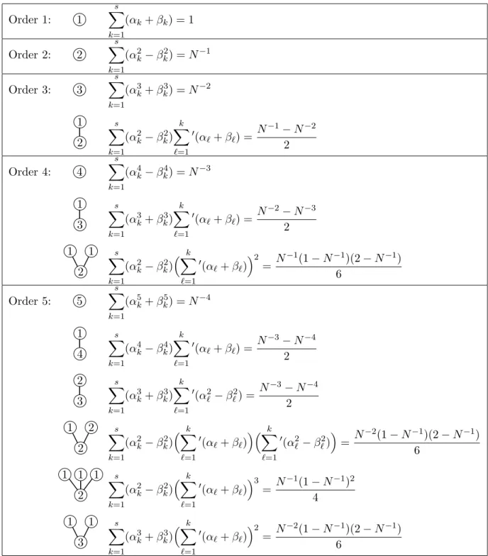
Table 1: Fifth-order conditions for MRCMs. The prime attached to a summation symbol indicates that the sum ofα^j_ℓ is only from 1 tok−1 while the sum of β^j_ℓ remains for 1 to k

. 2.2 Semi-discrete error analysis

Observe that by takingα_i =N⁻¹, β_i = 0,i= 1, . . . , N in (18) Lemma 2.1 immediately yields that the composition (ϕ_ε/N)^N(y) is again a B_∞-series

B∞(eN, ε, y) = (ϕ9 _ε/N)^N(y). (21)

Its coefficientse_N(τ) can be computed by using the following lemma.

Lemma 2.4. For all N ∈N^∗, the coefficientse_N(τ) of theB_∞-series in (21) satisfy

∀j∈N^∗, e_N( j ) =N^1−j,

∀τ = [τ1, . . . , τn]j ∈ T∞, N^kτkeN(τ) =

N−1X

k=1

k^{kτ1k+...+kτnk}e^′_k(τ).

Proof. With α_i = 1 andβ_i= 0, i= 1, . . . , N, Lemma 2.1 givesb_k(τ) =a_k−1(τ) and thus aN(τ) =

XN

k=1

a^′_k−1(τ) =

N−1

X

k=1

a^′_k(τ).

UsingB_∞(e_N, ε, y) =B_∞(a_N, ε/N, y) yields a_N(τ) =N^kτke_N(τ) and allows to conclude.

We obtain for instance e_N( 1 ) = 1, e_N( 2 ) =N⁻¹ and

e_N 1 1

= 1−N⁻¹

2 , e_N 2 1

= N⁻¹(1−N⁻¹)

2 , e_N

2 1 1

= N⁻¹(1−N⁻¹)(2−N⁻¹)

6 .

Now, recalling that the map ϕε can be interpreted as a consistent integrator for equation (3), (ϕ_ε/N)^N(y₀) converges to its solution z(ε) for N → ∞ and it is thus expected that the coefficients e_N(τ) converge to e_∞(τ) as N → ∞. This is shown in next proposition.

Proposition 2.5. The coefficients of theB_∞-series (21)satisfye_N(τ)→e_∞(τ)forN → ∞.

In particular, for N → ∞ the order conditions (24) coincide with the order conditions of standard composition methods (18) for the differential equation (3).

Proof. The proof is made by induction on |τ| and is a consequence of Lemma 2.4 and (20).

The result is clear for trees with one vertex using e_N( j ) = N^1−j. Given a tree τ = [τ₁, . . . , τ_n]_j ∈ T_∞, assume that the result is true for all tree u ∈ T_∞ with |u| < |τ|. By the induction assumption, we have e_k(τ₁)· · ·e_k(τ_n) → e_∞(τ₁)· · ·e_∞(τ_n) for k → ∞. Using the estimate PN−1

k=1 k^ℓ ∼ N^ℓ+1/(ℓ+ 1) for N → ∞ with ℓ = kτ1k+. . .+kτnk, we deduce using Lemma 2.4 that lim_n→∞e_N(τ) = e_∞(τ₁). . . e_∞(τ_n)/(ℓ+ 1) = e_∞(τ) for j = 1, and lim_n→∞e_N(τ) = 0 =e_∞(τ) for j >1, which concludes the proof.

Consider now theB∞-seriesB∞(a, ε, y) associated to a semi-discrete MRCM of the form (7) with H =ε. Writing the order conditions now boils down to comparing the coefficients of B_∞(a, ε, y) and B_∞(e_N, ε, y) and estimating the remainder term. Next lemma provides estimates of the derivatives of ϕ^N_ε w.r.t. ε. In order to alleviate the presentation, let us denote forρ >0,B_ρ(y₀) ={y ∈R^d;ky−y₀k ≤ρ}, and for a given functiony7→k(y) defined on B_ρ(y₀),

kkkρ:= sup

y∈Bρ(y0)

kk(y)k and k∂_yⁿkkρ:= sup

y∈Bρ(y0), kv_ik= 1, i= 1, . . . , n

k∂_yⁿk_ε(y) (v₁, . . . , v_n)k.

Note that if (y, ε) 7→ Θε(y) in (1) is of classC^p+1 with respect to (y, ε) on the compact set B_ρ(y₀)×[−ε0, ε₀], then there exist positive constantsK and L such that, for all |ε| ≤ε₀

k∂yϕ_εkρ≤1 +εL, ∀k= 2, . . . , p+ 1, k∂^k_yϕ_εkρ≤εL,

∀0≤k+l≤p+ 1, k∂_y^k∂^l_εϕ_εk_ρ≤K.

Lemma 2.6. Assume that (y, ε)7→Θ_ε(y) is defined and of class C^p+1 with respect to (y, ε) on B2R(y0)×[−ε0, ε0] for a given R >0 and a given ε0 >0. Then, there exists a constant H₀ such that for all εand N ≥1 withH =N ε≤H₀,

∂_ε^p+1ϕ^N_ε

R≤CN^p+1,

∂_H^p+1ϕ^N_H/N

R≤C, (22)

where C is independent ofN and ε.

Proof. For ˜y₀∈B_R(y₀) and denoting M := sup_|ε|≤ε0kΘεk2R, we have kϕ^N_ε (˜y₀)−y₀k ≤

XN k=1

kϕ^k_ε(˜y₀)−ϕ^k−1_ε (˜y₀)k+k˜y₀−y₀k ≤R+N εM

as long as the iterates ϕⁱ_ε(˜y₀) and ϕⁱ_ε(y₀) remain in B_2R(y₀) for 0 ≤ i ≤ N. Hence, if N ε≤ H0 := min(R/M, ε0) then kϕ^k_εkR ≤2R for all k = 0, . . . , N. Under this assumption, we now wish to prove by induction on n, that

∀n= 1, . . . , p+ 1,

∂_εⁿϕ^N_ε

R≤C_nNⁿ (23) for some constantsCn independent ofN, ε. Now, given a smooth functiong:B_2R(y0)→R^d of classC^p+1, Fa`a di Bruno’s formula reads

∂_ε^k(g◦ϕ^N_ε ) = X

m∈Nk, σ(m)=k

B_mg^(|m|)◦ϕ^N_ε

(∂_ε¹ϕ^N_ε )^m1, . . . ,(∂_ε^kϕ^N_ε )^mk

where the sum is over all multi-indices m = (m₁, . . . , m_k) of N^k such that k = σ(m) :=

P_k

j=1jm_j and where|m|denotesm₁+. . .+m_k and

B_m = k!

m₁!1!^m1· · ·m_k!k!^mk. We now use the differentiation formula

∂_εⁿ(ϕε◦ϕ^N_ε ) = Xn

k=0

n!

k!(n−k)! ∂^k_ε(∂_µ^(n−k)ϕµ◦ϕ^N_ε )

µ=ε

and takeg= ∂µ^(n−k)ϕµ

µ=ε in Faa di Bruno’s formula. This yields

∂_εⁿ(ϕ^N+1_ε ) = X

0≤k≤n, m∈N^k, σ(m) =k

n!

k!(n−k)!B_m

∂_y^|m|∂_ε^n−kϕ_ε

◦ϕ^N_ε

(∂_ε¹ϕ^N_ε )^m1, . . . ,(∂_εⁿϕ^N_ε )^mn

Hence, using the induction assumption, we get the estimates ∂_εⁿϕ^N+1_ε

R ≤ k∂_εⁿϕεk2R+ X

1≤k≤n−1, m∈N^k, σ(m) =k

n!

k!(n−k)! B_mk∂_y^|m|∂^n−k_ε ϕεk2R

Yk

j=1

k∂_ε^jϕ^N_ε k^m_R^j

+ X

m∈Nⁿ, σ(m) =n, mn= 0

B_mk∂_y^|m|ϕεk_2R Yn j=1

k∂_ε^jϕ^N_ε k^m_R^j +k∂yϕεk_2Rk∂_εⁿϕ^N_ε k_R

≤ K+KC˜_n

n−1X

k=1

N^k+εnCˆ_nLNⁿ+ (1 +εL)k∂_εⁿϕ^N_ε kR

≤ nKC˜_n(N+ 1)ⁿ⁻¹+nCˆ_nLH₀Nⁿ⁻¹+ (1 +εL)k∂_εⁿϕ^N_ε kR

≤ C¯_n(N+ 1)ⁿ⁻¹+ (1 +εL)k∂ⁿ_εϕ^N_ε kR

where the constants ˜C_n and ˆC_n are defined as C˜n= max

k=1,...,n−1

X

m∈Nk σ(m) =k

B_m Yk

j=1

C_j^mj and ˆCn= X

m∈Nⁿ⁻¹ σ(m) =n

B_m

n−1Y

j=1

C_j^mj

and ¯C_n =nmax(K, KC˜_n,Cˆ_nLH₀). Finally, using a standard discrete Gronwall lemma and H=N ε≤H0 yields

k∂_εⁿ(ϕ^N_ε )kR≤C¯_n XN

k=1

(1 +εL)^N−kkⁿ⁻¹≤C¯_nNⁿe^LεN ≤C¯_nNⁿe^LH0

which allows to conclude the proof of the first estimate in (22) by choosing Cn= ¯Cne^LH0 in (23). The second estimate is straightforwardly obtained through a change of variables.

We may now state the main result for the local error of the semi-discrete MRCM (7).

Theorem 2.7. Consider a semi-discrete MRCM (7) and assume further that its coefficients αi(N), βi(N), i= 1, . . . , sare bounded with respect to N for allN ≥N0 and satisfy

a(τ) =e_N(τ), for all τ ∈ H withkτk ≤p, (24) for a given order p≥1. Then, for all H ≤H₀,N ≥N₀,

kΨN,H−(ϕ_ε)^NkR≤CH^p+1 where H =N εand the constant C is independent of N, ε.

Proof. Consider the two B_∞-seriesB_∞(a, H, y) and B_∞(e_N, H, y) associated respectively to the semi-discrete MRCM (7) and toϕ^N_H/N(y) in (21). It follows from Theorem 2.3 that these B∞-series formally coincide up to order H^p. A Taylor expansion of ΨH(y)−(ϕ_H/N)^N(y) with integral remainder thus leads to

ΨN,H(y)−(ϕ_H/N)^N(y) = Z H

0

1

p!(H−s)^p ∂^p+1Ψ_s

∂s^p+1 (y)ds− Z H

0

1

p!(H−s)^p ∂^p+1ϕ^N_s/N

∂s^p+1 (y)ds.

The derivative^∂

p+1ϕ^N_s/N

∂s^p+1 is bounded by Lemma 2.6. Given that coefficientsαj, βjare uniformly bounded with respect to N, ^∂_∂s^p+1p+1^Ψs is bounded as well. We conclude using (ϕ_H/N)^N(y) =

(ϕε)^N(y).

We report in Table 1 order conditions up to order 5 as derived above. Note that Lemma 2.4 implies (by induction) that the value of N^kτke_N(τ) is independent of the labels of the nodes of a given tree τ ∈ T∞. This explains why similar right-hand sides e_N(τ) are obtained for trees where only labels differ. An immediate consequence of Proposition 2.5 is the following remark.

Remark 2.8. Notice that forN → ∞, the order conditions (24)reduce reduce to the classical order conditions of standard composition methods (18) for the approximation of the flow of ((3)).

2.3 Fully-discrete error analysis

In this subsection, we derive convergence estimates for fully-discrete MRCMs (16). We high- light once again that this is essential in view of applications because the exact computation of the mapϕ_ε is not available in general and has to be approximated by a map Φ_h,ε.

Theorem 2.9. Assume that the hypotheses of Theorem 2.7 are fulfilled. Consider a fully- discrete MRCM (16) where the basic map Φ_h,ε is assumed to satisfy the accuracy estimate (15) for given q and r. Then

kΨ_N,H,h−(ϕε)^NkR≤C(H^p+1+H^rh^q) where H =N ε,h≤εand the constant C is independent of N, ε, H, h.

As a consequence of Theorem 2.9, by standard arguments in the convergence analysis of one-step integrators, one gets a global error estimate for the numerical approximations y_m = Ψ_N,H,h(y_m−1) of problem (9) of the form

y_m−y(mH) =O(H^p+H^r−1h^q) for m H≤T.

For the proof of Theorem 2.9, we recall the following classical discrete Gronwall estimate.

Lemma 2.10. Let (φ_j, ψ_j), j= 1, . . . , k, be k couples of maps satisfying for ρ, ν >0 kφ_j(y)−ψ_j(y)k ≤ρ, kφ_j(y₁)−φ_j(y₂)k ≤(1 +ν)ky₁−y₂k, for all j= 1, . . . , k and all y, y1, y2. Then,

kφk◦ · · · ◦φ₁(y)−ψ_k◦ · · · ◦ψ₁(y)k ≤e^νkkρ.

Proof. Let a_j =φ_k◦ · · · ◦φ_k−j+1,b_j =ψ_j◦ · · · ◦ψ₁. We have a_k(y)−b_k(y) =

k−1X

j=0

a_k−j−1◦φj+1◦bj(y)−a_k−j−1◦ψj◦bj(y)

ka_k(y)−b_k(y)k ≤

k−1X

j=0

(1 +ν)^k−j−1kφj+1◦bj(y)−ψj+1◦bj(y)k ≤ke^νkρ where we used the estimatePk−1

j=0(1 +ν)^k−j−1 ≤Pk−1

j=0e^kjνk ≤kR1

0 e^νktdt≤ke^νk.

Proof of Theorem 2.9. We use the estimate

kΨN,H,h−(ϕ_ε)^NkR≤ kΨN,H,h−Ψ_N,HkR+kΨN,H−(ϕ_ε)^NkR

From Theorem 2.7, we have kΨN,H−(ϕ_ε)^NkR≤CH^p+1.The next estimate kΨN,H,h−Ψ_N,HkR≤CH^rh^q

is a consequence of Lemma 2.10 with k = 2s, ρ = CH^rh^q (using (15) with ε replaced by α_j(N)H and β_j(N)H), ν=O(ε) being a Lipsitz constant for the near-identity mapϕ_ε, and φ_2j−1=ϕ_αj(N)H,φ_2j =ϕ^∗_β

j(N)H,ψ_2j−1 = Φ_h,αj(N)H,ψ_2j = Φ^∗_h,β

j(N)H.

3 Effective construction of MRCMs

The simplest method of order 1 is obtained simplify for s= 1, α₁ = 1, β₁= 0 in (18), ϕ_H(y) =ϕ^N_ε (y) +O(H²).

For order 2, there exist a unique solution with s = 1, given by α₁ = (1 +N⁻¹)/2 and β₁ = (1−N⁻¹)/2,

ϕ_α1H ◦ϕ⁻¹_−β1H(y) =ϕ_(H+ε)/2◦ϕ⁻¹_{−(H−ε)/2}(y) =ϕ^N_ε (y) +O(H³).

For order 3, there do not exist real solutions with s = 2. We directly consider order 4, for which there are 7 order conditions to be satisfied. It turns out that there exists a family of solutions with s = 3, i.e. with only 6 free parameters α_j, β_j. We consider the following solution for N =∞ given by with

α₁ =β₁ =α₃ =β₃= 1

4−2·2^1/3, α₂ =β₂= 1

2 −2α₁.

The idea is then to setδ= 1/N and to search for continuous functionα_j(δ⁻¹), β_j(δ⁻¹) defined forδ ∈[0, N₀⁻¹] and which coincide with the above coefficients for δ = 0. This calculation is made by a continuation method.

However, it is known that for standard composition methods (N =∞), the composition methods with minimal number of compositions are not the most efficient in general. We thus increment the parametersand construct a family of MRCMs of orderp= 4 withs= 4 where we choose to minimize the sum of the squares of the coefficients. This yields the following optimization problem with constraints: find δ 7→ (αi(δ⁻¹), βi(δ⁻¹)), i = 1, . . . , s minimizing P_s

k=1(α_k(δ⁻¹)² +β_k(δ⁻¹)²) and fulfilling the order conditions up to order p. This is done using a standard optimization package. For a practical implementation, we consider a set of K = 33 Chebyshev points δ_k, k = 1, . . . , K sampling the interval [0, N₀⁻¹] and for which we compute the corresponding coefficients α_k(δ⁻¹_i ), β_k(δ_i⁻¹), k= 1, . . . , k. This calculation is made once for all and stored. We then use Chebyshev interpolation to recover the coefficients αi, βi for any value of δ= 1/N ∈[0, N₀⁻¹]. The numberK of sample points has been chosen to guaranty that the Chebyshev interpolation error is smaller than the machine precision.

Remark 3.1. Notice that multi-revolution composition methods with complex coefficients can also be considered (see [6, 16] in the context of standard composition methods). For instance, the fourth order conditions to achieve order3for a multi-revolution composition method have a complex solution for s= 2, given for all N ≥2 by:

α1(N) =α2(N) = 1 4+ 1

2N +i

p3−12/N²

12 , β1(N) =β2(N) = 1 4− 1

2N +i

p3−12/N²

12 .

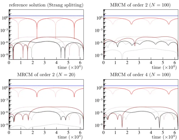
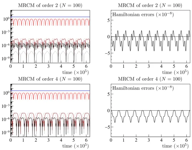
4 Numerical experiments

The aim of this part is to obtain a numerical confirmation of the orders of convergence given above and to demonstrate the efficiency of MRCMs. The first problem, which is a modification of the Fermi-Pasta-Ulam problem [12], is directly of the form (9) and serves classically in the literature as a test problem to measure the error behavior of the various

10¹ 10² 10³

10⁻⁹ 10⁻⁶ 10⁻³

10¹ 10² 10³

10⁻⁹ 10⁻⁶ 10⁻³

10¹ 10² 10³

10⁻⁹ 10⁻⁶ 10⁻³

10¹ 10² 10³

10⁻⁹ 10⁻⁶ 10⁻³ error inq₁

fnc evals

error inp₁

fnc evals error inq₂

fnc evals

error inp₂

fnc evals Figure 1: Problem (25) withη= 2⁻¹² and initial conditions (27). Errors of multi-revolution composition methods at time t = 2π as functions of the number of evaluations of ϕ_µ (for many values of the parameter N). Methods of orders 1 (circles), 2 (stars), 4 (s = 3 with white squares), 4 (s= 4 with black squares).

methods for integrating single-frequency highly oscillatory systems. The second test problem is borrowed from the PDE literature and requires to be discretized with a spectral method:

we aim with this example at illustrating the qualitative properties of MRCMs.

4.1 A Fermi-Pasta-Ulam like problem

In this subsection, we consider a problem taken from [15], which is a single-frequency mod- ification of the Fermi-Pasta-Ulam problem often used to test methods for highly-oscillatory problem. Its Hamiltonian function is given by

E_η(p, q) = 1 2

X6

i=1

p²_i + 1 2η²

X6

i=4

q_i²+V(q), (25)

with the quartic interaction potential V(q) = 1

4((q1−q4)⁴+ (q2−q5−q1−q4)⁴+ (q3−q6−q2−q5)⁴+ (q3+q6)⁴), whereη >0 is a small parameter.

In order to apply our MRCMs to that problem, we first rewrite the original Hamiltonian system into the format (9): we consider the family of Hamiltonian systems depending on the parameters ε, η >0 given as

H_ε,η(p, q) = 2π

ε F_η(p, q) + 2π S(p, q), (26)

where

Fη(p, q) = η 2

X6

i=4

p²_i + 1 2η

X6

i=4

q²_i and S(p, q) = 1 2

X3

i=1

p²_i +V(q).

Obviously, the original Hamiltonian system is recovered by considering ε= 2πη, that is Eη(p, q) =H2πη,η(p, q).

One can readily check that, for each fixed value of η, the family of Hamiltonian systems corresponding to the Hamiltonian functions (26) are of the form (9), with a 12×12 matrix A having 2πi, −2πi, and 0 as the only eigenvalues. For a given value of η >0, we consider the family of near-to-identity maps ϕ_ε defined as the flow with time ε of the Hamiltonian system associated to the Hamiltonian function (26). Then, the solutions y(t) = (p(t), q(t)) of the original Hamiltonian problem at times t = 2πηM for integer values of M are such thaty(2πηM) =ϕ^M_2πη(y(0)). Hence, the solutiony(t) = (p(t), q(t)) with a given initial value y(0) =y₀ can be approximated at multiplest_m =mH of H = 2πηN asy(t_m) ≈ Ψ^m_H,h(y₀), where ΨH,h is a fully-discrete MRCM (16) based on some computable approximation Φµ,h of ϕ_µ.

Recall thatϕ_µ is the flow with time 1 associated to the Hamiltonian functionµH_µ,η(p, q), so that a convenient choice of Φ_µ,h may be the composition ofnsteps of step-sizeh= 1/nof a splitting method applied to the splitting into fast and slow contributions

2π F_η(p, q;η) + 2πµ S(p, q)