Both test suites have been implemented in the COCO platform for benchmarking black-box optimization, and various visualizations of the test functions are shown to reveal their properties. The advantage of such an approach is that the analytical forms of the Pareto front and the Pareto set can be exploited to facilitate performance evaluation. In the special case where each of the two objective functions has a unique global minimum (that is, one point in the search space that maps to the global minimum value of the function), znadir= (fα(arg minfβ(x)), fβ (arg minfα( x))).
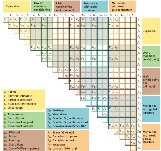
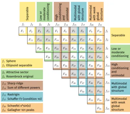
Similar to the single-objective bbob functions, the WFG suite of Huband et al. 2006) use problem transformations that change the properties such as (non-)separability, bias and the shape of the Pareto front of underlying raw objective functions. The optimum of the linear function is reached at a (randomly chosen) corner of the hypercube[−5,5]nand in the orthogonal beyond this point. 55 bioobjective functions for the finalbbob biobjsuite, indicated as F1toF55in the rest of the paper.
In the black-box optimization benchmarking setup of the COCO platform, the algorithm is allowed to use the values. Our proposed test functions are parameterized and their instances are instantiations of the underlying parameters of debbob functions (see Hansen et al., 2021)8.
The bbob-biobj-ext Test Suite
The bbob-biobj-ext Functions and Function Groups
As a result, we estimate the hypervolume of the Pareto set per instance and does not use the single-objective technique of aggregating results from different instances on simulated restarts (Hansen et al., 2021) to estimate runtimes to target values not achieved on a given instance. . The second reason to discard simulated restarts in the multiobjective case is the performance evaluation setup in COCO: we measure performance based on the entire archive of all solutions evaluated so far. However, runs on different instances produce incompatible archives, and thus simulated restarts cannot account for the hypervolume achieved by previous runs.
To better understand the functions in thebbob-biobjandbbob-biobj-ext-suites, we visualize and analyze their properties. We present their most famous Pareto set and Pareto front approximations along with 1-dimensional search space slices in Section 6.1, investigate a necessary optimality condition in Section 6.2, and provide 2-dimensional dominance-based (Section 6.3) and gradient-based plots ( Section 6.4 ) known from the literature for all proposed functions.
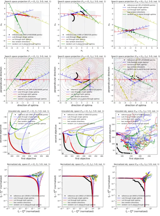
Plots of Pareto Set and Front Approximations
Pareto sets and Pareto front approximations in Figure 3 are downsampled so that only one solution is shown per grid point - with a precision of 2 decimal places for the search space plots and 3 decimal places for the objective space plots to define the grid. The number of all available and actually displayed solutions is given in the legend of each plot. An important question to ask is whether our collected Pareto set approximations are qualitatively good, i.e. how close they are to the true Pareto front.
For our blackbox functions, we estimate collinearity as follows: for each Pareto set approximation (or function instance), we evaluate the two objective function gradients of solutions by finite (central) differences and calculate the angle between them. The angle between the gradients is closely related to the normalized multiobjective gradient of Kerschke and Grimme (2017), in the biobjective case defined as. The length of the normalized biobjective gradient(1) and the cosine of the angle between the two gradients, say vandw, are related as follows. 2) The proof is given in Appendix B.
17Use a step length of ε = 10−8 to approximate the ith coordinate of the gradient inx ∈ Rn with. 18Only every hundredth point of the Pareto set approximations is shown to reduce computation time and file size. The legends in Figure 4 show the number of points displayed compared to the full size of the Pareto set approach for each dimension and for the last instance.
For smooth functions, this also suggests that our approximations of Pareto sets are reasonably close to a true local Pareto set. On the other hand, there are functions with higher values of 1 + cos(α), indicating (at first glance) that the approximations of the Pareto set are less converged. We have verified that for the combination of sphere and sharp ridge, all solutions in our Pareto array approximation lie along a line between two single-objective optima, but that depending on which side of the sharp ridge a point is located, the two target gradients are directed in the same or opposite direction, resulting in small and large values of 1 + cos(α), respectively.
Although we do not know the exact Pareto set for the proposed functions (except for the double-sphere functionF1= (f1, f1)), the generated non-dominated Pareto set approximations appear to be accurate enough, also based on consistency: both, the large amount of non-dominated solutions of various algorithms, implemented by various authors as presented here, and the non-dominated solutions on a 2-dimensional grid, as presented in the next subsection, show qualitatively the same sets19.
Dominance-Based Plots
This also applies to other combinations of targets, such as sphere/sum of various powers functionF6 = (f1, f14), sphere/Schwefel functionF9 = (f1, f20), attractive sector/sum of various powers functionF23 = ( f6, f14), dual function sums of different powers F41 = (f14, f14) and dual Schwefelxsinx function F53 = (f20, f20) and with slightly higher cosine values for several other functions, for example attractive sector/Gallagher 101 peaks functionF27 = (f6, f21) and dual original Rosenbrock functionF28= (f8, f8). Two examples, the sphere/sharp ridge function F5= (f1, f13) and the original Rosenbrock/sharp ridge function F29= (f8, f13), are shown in Figure 4. A closer look at the functions with the (strongest) right shift in the ECDF reveals, that often one of the targets is multimodal, flat, or its gradient does not change smoothly (which is the case for the sharp ridge function in Figure 4).
Especially in the latter case, we do not expect the values of 1 + cos(α) to be close to zero. Based on solutions on a regular grid in the search space, the dominance ratio of each grid point is the ratio of all grid points that dominate it. The plot uses a logarithmic color scale, with the common non-dominated points shown in yellow.
The non-dominated grid points are shown in the second row of Figure 5 in black, along with the first and second target level clusters in blue and red. In dark green, we show all network points P for which all 8 neighboring network points (in the Moore neighborhood) are mutually non-dominated in P. In terms of landscape analysis, we can call the regions of greens in plots "dominant neutral local optima regions" (Fieldsend et al., 2019) in the sense that a dominance-based climber will be able to explore a green. non-dominated single motion region.
The pink regions consist of grid points for which at least one neighboring grid point dominates it, and all dominant movement paths from neighbors in pink regions lead to the same green region (Fieldsend et al., 2019). Each pink area is considered a "pool of attraction" of a green area in the sense that a local dominance-based hillclimber can only move towards the included green area. Finally, a grid point is assigned a white color if at least two of its dominant neighbors belong to two different basins of attraction—white areas in the plots therefore show the boundaries between the basins.
The existence of multiple, different basins of attraction can be interpreted as multimodality of a multi-objective problem: it is called unimodal if and only if a single basin of attraction is present (and thus no two different local Pareto-optimal sets exist).

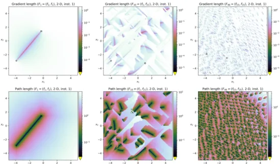
Gradient-Based Plots
Summary of Observed Problem Properties
First row: pure gradient length at each grid point, Second row: the length of the path from each grid point towards the next local optimum (see text for more information). First, different instances of the same function most of the time share the same properties—especially for the number of basins of attraction and the Pareto front convexity. Similarly, 78 of the 92 bbob-biobj-ext features do not differ among instances 1–5 with respect to Pareto set/front (dis-)continuity—only the number of connected Pareto set/front parts changes in case discontinuities are observed .
Out of 92 bbob-biobj-extfunctions, only 27 (of which 18 belong to 55 bbob-biobjsuite) have a continuous Pareto front and a continuous Pareto set in all five cases (i.e., therefore, we conclude that most of the proposed functions have challenging Pareto set and Pareto front shapes Moreover, the Pareto set of most problem instances of the proposed test suites is within the hyperfield [−5,5]n.
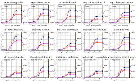
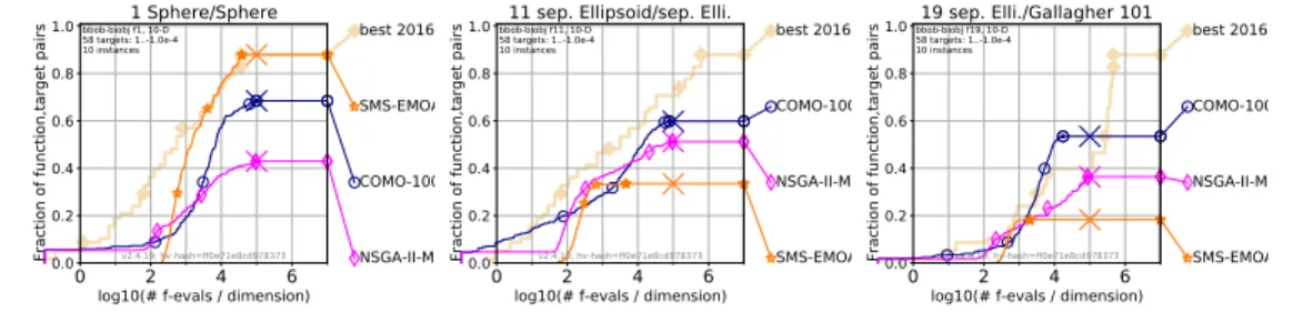
Otherwise, performance is measured as minus the minimum distance of any solution found (in objective space and normalized as above) to the box [0,1]2, for details see (Brockhoff et al., 2016). Qualitative differences in performance behaviors between algorithms remain similar even within function groups, while differences are smaller in groups that include multimodal objective functions. Finally, in the right graph, we note that COMO-100 matches and exceeds the performance of the best 2016 benchmark algorithm on the ellipsoid/Gallagher peak function 101 F19 = (f2, f21) for budgets between 5·103 and 104 times dimension evaluations, but also doesn't get better soon after.
Consistent with the concepts of the single-objective bbob test suite, we propose two concrete bi-objective test suites based on the idea of combining (subsets of) the existing bbob single-objective functions. 24 Shown is the performance of the three algorithms COMO-CMA-ES with a population size of 100 ("COMO-100", Tour´e et al. The disadvantage of unknown analytical forms of Pareto sets and Pareto fronts in our proposal is addressed by to collect the non-dominated solutions from extensive experiments with dozens of different optimization algorithms and provide and visualize the Pareto set and Pareto front approximations for each problem.
This leads to long run times for the benchmarking experiment and, more importantly, discourages routinely investigating new results for each feature individually. This work was supported by grant ANR-12-MONU-0009 (NumBBO) from the French National Research Agency. The impact of variational operators on the performance of SMS-EMOA on the bi-objective BBOB-2016 test suite.
Real-World Function Properties
Balancing Problem Difficulties
Function Instances
Normalization and Target Difficulties