Numerical observers with vanishing viscosity for the 1d wave equation

HAL Id: hal-00914924

https://hal.archives-ouvertes.fr/hal-00914924

Submitted on 10 Dec 2013

HAL is a multi-disciplinary open access archive for the deposit and dissemination of sci- entific research documents, whether they are pub- lished or not. The documents may come from teaching and research institutions in France or abroad, or from public or private research centers.

L’archive ouverte pluridisciplinaire HAL, est destinée au dépôt et à la diffusion de documents scientifiques de niveau recherche, publiés ou non, émanant des établissements d’enseignement et de recherche français ou étrangers, des laboratoires publics ou privés.

Numerical observers with vanishing viscosity for the 1d wave equation

Galina Garcia, Takéo Takahashi

To cite this version:

Galina Garcia, Takéo Takahashi. Numerical observers with vanishing viscosity for the 1d wave equation. Advances in Computational Mathematics, Springer Verlag, 2014, 40 (4), pp.711-745.

�10.1007/s10444-013-9320-5�. �hal-00914924�

Numerical observers with vanishing viscosity for the 1d wave equation

Galina Garc´ıa^∗, Tak´eo Takahashi^†‡§

July 7, 2013

Abstract

We consider a numerical scheme associated with the iterative method developed in [34] to recover initial conditions of conservative systems. In this method, the initial conditions are reconstructed by using observers. Here we use a finite-difference discretization in space of these observers and our aim is to prove estimates of the errors with respect to the mesh size and to the number of steps in the iterative method. This is done in the particular example of the 1d wave equation. In order to avoid restrictions of the number of steps with respect to the mesh size, we add a numerical viscosity in the numerical observers. A generalization for other equations is also given.

1 Introduction and main results

The aim of this article is to consider and analyze an iterative method based on observers to reconstruct initial conditions of some evolution equations. More precisely, we focus on a method developed in [34]

to recover the initial conditions for reversible infinite-dimensional systems. Our aim is to analyze this method when we discretize the evolution equations. In order to do this, we recall the method considered in [34] for a 1d wave equation and we then discretize this equation by using the finite difference method on a uniform mesh. Nevertheless, our approach can be extended to other systems and to other numerical discretization methods (see Section 7).

Let us consider the 1d wave equation:











∂_ttv−∂_xxv= 0 in (0, τ)×(0,1),

v(t,0) = 0 fort∈(0, τ),

∂_xv(t,1) = 0 fort∈(0, τ), v(0, x) =v⁰(x), ∂_tv(0, x) =v¹(x) for x∈(0,1).

(1)

It is well-known that system (1) is well-posed for

(v⁰, v¹)∈H_L¹(0,1)×L²(0,1), (2) where

H_L¹(0,1) :=

v∈H¹(0,1) ; v(0) = 0

(see, for instance, [5] for the definitions of the Lebesgue and the Sobolev spaces). In particular, for initial conditions satisfying (2), there exists a unique solutionv of system (1) verifying

v∈C([0, τ];H_L¹(0,1))∩C¹([0, τ];L²(0,1)).

∗Departamento de Matem´atica y Ciencia de la Computaci´on, Universidad de Santiago, Casilla 307, Correo 2, Santiago, Chile (galina.garcia@usach.cl)

†Inria, Villers-l`es-Nancy, F-54600, France (takeo.takahashi@inria.fr),

‡Universit´e de Lorraine, IECN, UMR 7502, Vandoeuvre-l`es-Nancy, F-54506, France,

§CNRS, IECN, UMR 7502, Vandoeuvre-l`es-Nancy, F-54506, France,

Moreover, if we define the observation y by

y(t) :=∂_tv(t,1) fort∈(0, τ), (3) then, from the admissibility of the observation operator (see, for instance, [37]), we have

y∈L²(0, τ).

The corresponding inverse problem consists in recovering the initial data (v⁰, v¹) of (1) by using the observationy defined by (3), where τ is a positive time to be determined.

In order to solve this inverse problem, Ramdani, Tucsnak and Weiss propose in [34] an iterative algorithm. They define the two following forwardand backward operators F_y,B_y:

F_y :H_L¹(0,1)×L²(0,1)→H_L¹(0,1)×L²(0,1), (q⁰, q¹)7→(q(τ), ∂_tq(τ)), (4) where











∂_ttq−∂_xxq = 0 in (0, τ)×(0,1),

q(t,0) = 0 fort∈(0, τ),

(∂xq+∂tq)(t,1) =y(t) fort∈(0, τ), q(0, x) =q⁰(x), ∂_tq(0, x) =q¹(x) forx∈(0,1),

(5)

and

B_y :H_L¹(0,1)×L²(0,1)→H_L¹(0,1)×L²(0,1), (q⁰_b, q¹_b)7→(q_b(0), ∂_tq_b(0)), (6) where











∂ttq_b−∂xxq_b= 0 in (0, τ)×(0,1),

q_b(t,0) = 0 fort∈(0, τ),

(∂_xq_b−∂_tq_b)(t,1) =−y(t) fort∈(0, τ), q_b(τ, x) =q⁰_b(x), ∂tq_b(τ, x) =q_b¹(x) for x∈(0,1).

(7)

Then, they consider the sequences

a⁽ⁿ⁾, b⁽ⁿ⁾

= (B_y ◦F_y)

a⁽ⁿ⁻¹⁾, b⁽ⁿ⁻¹⁾

, n∈N^∗, (8)

where a⁽⁰⁾, b⁽⁰⁾

is an initial guess of (v⁰, v¹).

The convergence analysis developed in [34] shows that forτ large enough, the sequence a⁽ⁿ⁾, b⁽ⁿ⁾ converges towards (v⁰, v¹). More precisely, we have the following result:

Proposition 1.1. Forτ >2, there exists α∈(0,1) such that for all n∈N,

a⁽ⁿ⁾−v⁰

2

HL¹(0,1)+

b⁽ⁿ⁾−v¹

2

L²(0,1)6α²ⁿ

a⁽⁰⁾−v⁰

2

HL¹(0,1)+

b⁽⁰⁾−v¹

2 L²(0,1)

. (9) Although the proof of the above proposition is a consequence of the general results of [34], we give it in Section 2 since it is quite short in our case and contains hints for the proof of the main result.

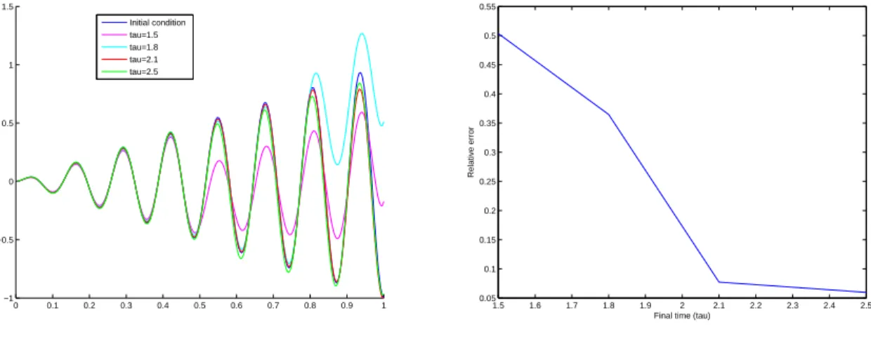
Let us note that the conditionτ >2 is related to the exact observability of (1) with the observation (3). Indeed, (1), (3) is exactly observable if and only if τ > 2. For the wave equation in dimension N > 1, the time τ is related to “Geometric Control Condition” (see [3]). We recall that exact observability is related to exact controllability and to stabilization property (see [21], [37]).

In this paper, we focus on the discretized counterpart of the above result. LetN ∈N and h= 1

N+ 1. (10)

We consider the uniform subdivision of (0,1): x_j = jh, j = 0, . . . ,(N + 1). Finally, we consider a positive constantν that is used in the numerical scheme to add a numerical viscosity.

The numerical adaptation of the method of [34] is given below. First, we consider spatial approx- imations of theforward and backward operators:

F_y,h:R^N+2×R^N+2 →R^N+2×R^N+2, (q_h⁰, q¹_h)7→(q_h(τ), q^′_h(τ)), (11) whereq_h= (q_j)₀6j6N+1 verifies















q_j^′′−q_j+1−2q_j +q_j−1

h² −ν

q^′_j+1−2q_j^′ +q_j−1^′

= 0 in (0, τ),16j6N,

q₀ = 0 in (0, τ),

q_N+1−q_N

h +q^′_N+1=y in (0, τ),

qj(0) =q⁰_j, q_j^′(0) =q¹_j forj= 0,· · · , N + 1,

(12)

and

B_y,h:R^N+2×R^N+2 →R^N+2×R^N+2, (q_b,h⁰ , q¹_b,h)7→(q_b,h(0), q_b,h^′ (0)), (13) whereq_b,h= (q_b,j)₀6j6N+1 verifies















q_b,j^′′ −q_b,j+1−2q_b,j+q_b,j−1

h² +ν

q_b,j+1^′ −2q^′_b,j+q_b,j−1^′

= 0 in (0, τ),16j 6N,

q_b,0 = 0 in (0, τ),

q_b,N+1−q_b,N

h −q_b,N+1^′ =−y in (0, τ),

q_b,j(τ) =q⁰_b,j, q_b,j^′ (τ) =q¹_b,j forj= 0,· · · , N+ 1.

(14)

Recall that y(t) =∂tv(t,1) is the observation of the system (1) defined by (3).

The terms −ν

q_j+1^′ −2q_j^′ +q_j−1^′

in (12) and +ν

q_b,j+1^′ −2q_b,j^′ +q_b,j−1^′

in (14) are numerical viscosities that play crucial role in our analysis. The idea of adding numerical viscosities in the numerical schemes for the wave equation was already considered by [35], [33], [31], [29], etc. They use these viscosities to obtain uniform observability or stabilization properties for the discretization of the wave equation. Without these viscosities, these properties may fail because of some spurious modes which are not well approximated ([2], [17], [18], etc.). Here, to reconstruct the initial conditions, a key point in the method is to have a uniform decay of the energy in time τ and this property is strongly related to the stabilization, which explain that we also add some numerical viscosity in the above systems. The change of sign is simply coming from the method proposed in [34], where both the forward and the backward steps need these uniform decay of the energy.

Using these operatorsF_y,hand B_y,h, we can recover the approximations ofv⁰ andv¹ by using the following sequences:

a⁽ⁿ⁾_h , b⁽ⁿ⁾_h

= (B_y,h◦F_y,h)

a⁽ⁿ⁻¹⁾_h , b⁽ⁿ⁻¹⁾_h

, n∈N^∗,

where

a⁽⁰⁾_h , b⁽⁰⁾_h

is an initial guess of (v⁰_h, v¹_h).

Our main result is

Theorem 1.2. Assume thatv⁰∈H²(0,1)∩H_L¹(0,1) and thatv¹ ∈H_L¹(0,1). Forτ >2and forν >0, there exists γ=γ(τ, ν)∈(0,1) such that for all N ∈N(and h given by (10)) and for all n∈N,

h 2

N

X

j=0





b⁽ⁿ⁾_j −v_j¹2

+ a⁽ⁿ⁾_j+1−a⁽ⁿ⁾_j

h −v_j+1⁰ −v_j⁰ h

!²

+νh² 2

b⁽ⁿ⁾_N+1−v¹_N+12

6 1

1−γ²ε_h+γ²ⁿ



 h 2

N

X

j=0





b⁽⁰⁾_j −v¹_j2

+ a⁽⁰⁾_j+1−a⁽⁰⁾_j

h −v⁰_j+1−v⁰_j h

!²

+νh² 2

b⁽⁰⁾_N+1−v_N+1¹ 2



, (15)

where v_j⁰=v⁰(jh), v¹_j =v¹(jh) for 06j6N + 1and where ε_h =ε_h

kv⁰k_H²_(0,1)∩H¹

L(0,1),kv¹k_H¹

L(0,1)

is independent of nand goes to 0 as h→0.

Remark 1.3. In the above result, let us note that in (15) h

2

N

X

j=0





b⁽ⁿ⁾_j −v¹_j2

+ a⁽ⁿ⁾_j+1−a⁽ⁿ⁾_j

h −v⁰_j+1−v⁰_j h

!²



is a discrete counterpart of

b⁽ⁿ⁾−v¹

2

L²(0,1)+

a⁽ⁿ⁾−v⁰

2 HL¹(0,1)

in (9). The term _1−γ¹2ε_h is independent of the number of iterations and can only be reduced by decreasingh, whereas the other term in the right-hand side of (15) goes to 0 if the number of iterations goes to infinity.

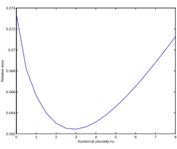
Remark 1.4. It is important to notice that the numerical viscosity we use in our numerical scheme allows to obtain in the above result a time τ and a decay γ independent ofh.

Remark 1.5. In Theorem 1.2, we need the following regularity on the initial conditions: v⁰ ∈ H²(0,1)∩H_L¹(0,1) and v¹ ∈ H_L¹(0,1). In particular, we need more regularity than in Proposition 1.1. This assumption allows us to deal with the numerical error for the observation (at the boundary), and it is not clear that it is possible to obtain (15) for v⁰ ∈ H_L¹(0,1) and v¹ ∈L²(0,1). For locally distributed observation, we would obtain the result for v⁰ ∈H₀¹(0,1) andv¹∈L²(0,1).

Let us make some comments on the main result. We consider here a finite difference approximations of the iterative algorithm proposed by [34]. This algorithm use back and forth in time observers to reconstruct the initial conditions. The use of observers is classical in finite dimensional systems (see, for instance, [20] ) and has been tackled in infinite dimensional systems ([1], [4], [6], [7], [9], [30], [10], [19], [22], [25]). The algorithm using back and forth in time observers for finite dimensional systems was considered in [15].

The method we use here could be adapted to other systems (Schr¨odinger equation, plate equation, Maxwell system, etc.) Instead of adding a vanishing viscosity, we could use one of the several methods which have been developed in the literature to handle the high frequency spurious modes: Tychonoff regularization [11], mixed finite elements [2], filtering of high frequencies [18], [24], etc. (see the review paper [38] for more details and extensive references). Let us note that in [8], the authors, prove that for regular solutions, the numerical viscosity is not needed. We present in Section 7 some possible generalizations of the studied done for the 1d wave equation.

It is important to notice that our work is related to another approach of this problem developed in [16]. In that case, the authors don’t add any vanishing viscosity and analyze the corresponding convergence of the numerical observers towards the initial conditions. The main differences with our work are that in their cases, the initial data are more regular and the observability operator is bounded with an extra hypothesis of regularity. Indeed their proofs, based on finite element method, consists in using these regularity assumptions to derive estimates errors and to follow the result obtain in the continuous system. In particular, it allows them to treat with the same approach a large class of systems and also to obtain similar results for the full-discretized case.

Here, we work directly on the discrete systems, and thus we don’t need such assumptions on the regularity of the initial conditions. In fact, we could adapt our work to the case of internal

observation and in that case, we could work with initial condition only in H₀¹(0,1)×L²(0,1) instead of

H²(0,1)∩H₀¹(0,1)

×H₀¹(0,1). Another difference with the result of [16] is that in their case, they need to choose a particular number of steps in the iterative method with respect to the mesh size.

Here, since we add this numerical viscosity, such a relation is not needed.

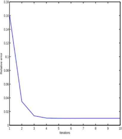
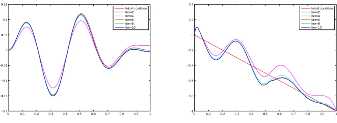
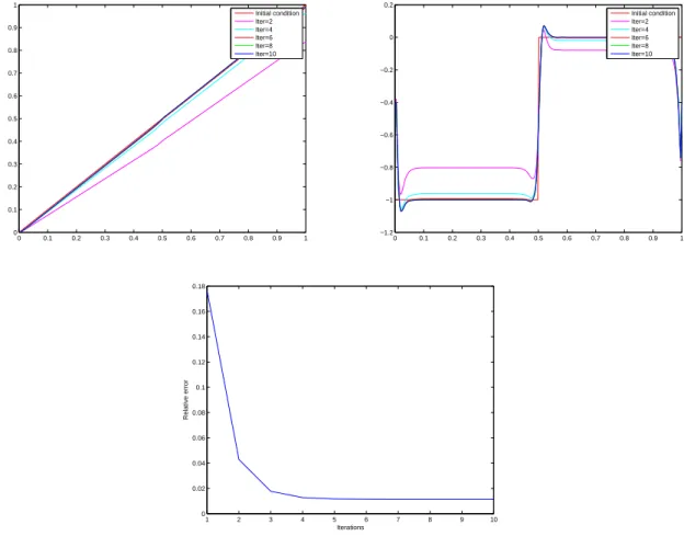
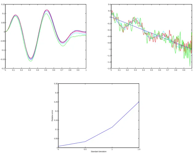
The paper is organized as follows: in Section 2, we present a short proof of Proposition 1.1. An important ingredient to obtain this result is the study of a damped wave equation. The discretization of this damped wave equation is analyzed in Section 3. Then Section 4 is devoted to some properties of the numerical schemes associated to (1) if we add a numerical viscosity. We study in particular the convergence results and an admissibility property. This allows to prove Theorem 1.2 in Section 5. Section 6 gives some numerical examples of this method. Finally, Section 7 presents some possible extensions of the result obtained for the 1d wave equation to more general systems.

2 Analysis in the theoretical framework

This section is devoted to the proof of Proposition 1.1. This analysis is already done in [34], but here we precise some aspects which help to understand the numerical analysis of the next section. Let us first consider the following damped wave equation.











∂_ttw−∂_xxw= 0 in (0,∞)×(0,1),

w(t,0) = 0 fort∈(0,∞),

(∂xw+∂tw)(t,1) = 0 fort∈(0,∞), w(0, x) =w⁰(x), ∂_tw(0, x) =w¹(x) forx∈(0,1).

(16)

Then we have the following classical result:

Lemma 2.1. Assume τ > 2. Then there exists α ∈ (0,1) such that for all w⁰, w¹

∈ H_L¹(0,1)× L²(0,1),

kw(τ)k²_H¹

L(0,1)+k∂_tw(τ)k²_L2(0,1)6α w⁰

2

HL¹(0,1)+ w¹

2 L²(0,1)

. (17)

Remark 2.2. The proof we give for this lemma is classical and is based on the multiplier method (see, for instance, [21]). It is used to obtain stabilizability properties. We recall the proof here since we use a similar method in the numerical case. Let us also notice that this method can be used to prove the same result for the wave equation in several dimensions (see, for instance, [37]). For interior domain measurements, the same result can be obtained again by using a multiplier method but a compactness argument is needed (see [23] for the continuous case, [35] for the discretized case).

Proof. We first multiply the first equation of (16) by ∂_twand integrate over (0,1):

d dt

1 2

Z 1 0

h(∂_tw)²+ (∂_xw)²i

dx−∂_xw(1)∂_tw(1) = 0,

using the third equation in (17) we obtain d

dt 1 2

Z ₁

0

h

(∂_tw)²+ (∂_xw)²i

dx+ (∂_tw)²(1) = 0, (18)

which implies in particular that the energy E = 1

2 Z ₁

0

h(∂_tw)²+ (∂_xw)²i

dx (19)

is a nonincreasing function of time.

Then we multiply the first equation of (16) byx∂_xw, integrate over (0,1) and after some compu- tation, we deduce

d dt

Z 1 0

∂twx∂xw dx− Z 1

0

x∂x(∂tw)² 2 dx−

Z 1 0

x∂x(∂xw)²

2 dx= 0.

The above equation implies d dt

Z 1 0

(∂tw)x(∂xw) dx−(∂tw)²(1) +E(t) = 0. (20) Let us set

Vε(t) :=E(t) +ε Z 1

0

∂tw(t)x∂xw(t) dx. (21)

We deduce from (18) and (20) that

V_ε^′(t) = (ε−1)(∂tw)²(1)−εE(t). (22) On the other hand, we have that

Z 1 0

∂_twx∂_xw dx

6E, which implies that

(1−ε)E6Vε6(1 +ε)E. (23)

Combining the above equation and (22) yields that forε∈(0,1), V_ε^′(t)6− ε

1 +εVε(t) for all t>0.

We deduce from the above equation and (23) that E(t)6 1 +ε

1−εexp

− ε 1 +εt

E(0). (24)

Let us consider the function

f(ε) := 1 +ε ε ln

1 +ε 1−ε

.

Forτ > f(ε), we have

α:= 1 +ε 1−εexp

− ε 1 +ετ

<1,

which implies (17). Since lim_ε→0⁺f(ε) = 2, we conclude the proof of the lemma.

Using the above result, we deduce the proof of Proposition 1.1:

Proof of Proposition 1.1. Let us setw=v−q wherevand q are respectively the solutions of (1) and (5). Then it can be easily checked thatwis the solution of (16) with the initial conditionsw⁰ =v⁰−q⁰ and w¹ =v¹−q¹. As a consequence, using Lemma 2.1, we deduce that forτ >2,

kv(τ)−q(τ)k²_H1

L(0,1)+k∂_tv(τ)−∂_tq(τ)k²_L2(0,1)6α

v⁰−q⁰

2

HL¹(0,1)+

v¹−q¹

2 L²(0,1)

. (25) Now let us set ˜w=v−q_b wherev andq_b are respectively the solutions of (1) and (7). Then it can be easily checked that ˜wis the solution of











∂_ttw˜−∂_xxw˜= 0 in (0,∞)×(0,1),

˜

w(t,0) = 0 fort∈(0,∞),

(∂_xw˜−∂_tw)(t,˜ 1) = 0 fort∈(0,∞),

˜

w(τ, x) =v(τ, x)−q⁰_b(x), ∂_tw(τ, x) =˜ ∂_tv(τ, x)−q_b¹(x) for x∈(0,1).

(26)

Thus,w(t, x) := ˜w(τ−t, x) satisfies (16) withw⁰(x) =v(τ, x)−q_b⁰(x) and withw¹(x) =−∂_tv(τ, x) + q_b¹(x). As a consequence, using Lemma 2.1, we deduce that forτ >2,

kv(0)−q_b(0)k²_H¹

L(0,1)+k∂_tv(0)−∂_tq_b(0)k²_L2(0,1)6α

v(τ)−q_b⁰

2

H¹L(0,1)+

∂_tv(τ)−q_b¹

2 L²(0,1)

. (27) In particular for (q_b⁰, q_b¹) = (q(τ), ∂_tq(τ)) =F_y(q⁰, q¹), we deduce from (25) and (27) that

v⁰−q_b(0)

2

HL¹(0,1)+

v¹−∂_tq_b(0)

2

L²(0,1) 6α²

v⁰−q⁰

2

HL¹(0,1)+

v¹−q¹

2 L²(0,1)

. (28) Consequently, we deduce that

(v⁰, v¹)−B_y◦F_y(q⁰, q¹)

2

HL¹(0,1)×L²(0,1) 6α²

(v⁰, v¹)−(q⁰, q¹)

2

H¹L(0,1)×L²(0,1)

and by induction, we deduce (9).

3 Numerical analysis of a damped wave equation

In order to prove Theorem 1.2, we first need, as in the theoretical part, to analyze a damped wave equation. More precisely, let us first consider the following finite-difference discretization of system (16) with the presence of a “pertubation”η=η(t) at x= 1:



















w^′′_j −w_j+1−2w_j+w_j−1

h² −ν

w_j+1^′ −2w^′_j+w_j−1^′

= 0 in (0, τ),16j 6N,

w₀ = 0 in (0, τ),

w_N+1−w_N

h +w_N^′ ₊₁=η in (0, τ),

w_j(0) =w⁰_j, w^′_j(0) =w¹_j 06j6N + 1.

(29)

The above system, with the add of the numerical viscosity term −ν

w^′_j+1−2w_j^′ +w^′_j−1

and in the caseη ≡0, was studied in [36]. They show the uniform exponential stability of the above system.

Here we prove a uniform decay of the energy with presence of the perturbationη.

Let us define the following energy associated to the system (29):

E_h(t) = h 2

N

X

j=0

"

w^′_j(t)2

+

w_j+1(t)−w_j(t) h

2# +νh²

2 w_N^′ ₊₁(t)2

. (30)

Lemma 3.1. The energy E_h defined by (30) satisfies E_h^′ =−(w^′_N+1)²−hν

N

X

j=0

w_j+1^′ −w^′_j2

+ηw_N^′ ₊₁+h²νη^′w_N^′ ₊₁ (31) in (0,∞).

Proof. In what follows, we use the classical formula (Abel transformation)

N

X

j=1

(b_j−b_j−1)a_j =b_Na_N+1−b₀a₀−

N

X

j=0

b_j(a_j+1−a_j). (32)

Applying (32), we deduce the following relations:

N

X

j=1

(w_j+1−2w_j +w_j−1)w^′_j =

N

X

j=1

[(w_j+1−w_j)−(w_j−w_j−1)]w^′_j

= (w_N+1−w_N)w^′_N+1−(w₁−w₀)w₀^′ −

N

X

j=0

(w_j+1−w_j)(w^′_j+1−w_j^′), and

N

X

j=1

(w^′_j+1−2w^′_j+w^′_j−1)w^′_j =

N

X

j=1

[(w_j+1^′ −w^′_j)−(w^′_j−w_j−1^′ )]w_j^′

= (w^′_N+1−w_N^′ )w_N^′ ₊₁−(w^′₁−w^′₀)w^′₀−

N

X

j=0

(w^′_j+1−w^′_j)².

Then, we multiply the first equation of (29) by hw_j^′, and by using the two above formulas, we obtain

h 2

N

X

j=1

d dt w^′_j2

−w^′_N+1(w_N+1−w_N)

h +h

N

X

j=0

(wj+1−wj)(w_j+1^′ −w^′_j) h²

−hν(w^′_N+1−w^′_N)w^′_N+1+hν

N

X

j=0

(w_j+1^′ −w^′_j)²= 0

The above equation, combined with the boundary condition in (29), yields h

2

N

X

j=0

d dt

"

w^′_j2

+

w_j+1−w_j h

2# +hν

N

X

j=0

w^′_j+1−w_j^′2

+ (w_N^′ ₊₁)²−ηw^′_N+1 +1

2h²ν d

dt w^′_N+12

−h²νη^′w^′_N+1 = 0, which implies (31).

The previous lemma shows that, without the “perturbation”η, the functionE_h is a nonincreasing function of time. We improve this result in the following lemma.

Lemma 3.2. Assume τ >2. Then there exist β∈(0,1) and C=C(ν) such that E_h(τ)6βE_h(0) +C

Z τ 0

η²+h²(η^′)²

ds. (33)

Proof. Let us define the following function of time W_ε:=E_h+ε

N

X

j=1

w_j^′jhw_j+1−w_j−1

2 −εh

4 w^′_N+12

. (34)

From (31) and the first equation of (29), we have W_ε^′ =−(w^′_N+1)²−hν

N

X

j=0

w_j+1^′ −w^′_j2

+ηw_N^′ ₊₁+h²νη^′w^′_N+1

+ε

N

X

j=1

w_j+1−2w_j +w_j−1

h² jhw_j+1−w_j−1

2 +ε

N

X

j=1

ν w^′_j+1−2w_j^′ +w^′_j−1

jhw_j+1−w_j−1 2 +ε

N

X

j=1

w_j^′jhw_j+1^′ −w^′_j−1

2 −εh

2 w^′_N+1w^′′_N+1. (35) First, using (32) and the third equation of (29), one obtains

ε

N

X

j=1

w_j+1−2w_j +w_j−1

h² jh

w_j+1−w_j−1 2

= ε

2h

N

X

j=1

j

[w_j+1−w_j]²−[w_j−w_j−1]²

= ε

2

w_N+1−w_N h

2

−εh 2

N

X

j=0

w_j+1−w_j h

2

= ε

2(η−w^′_N+1)²−εh 2

N

X

j=0

w_j+1−w_j h

2

. (36) Second, we have

ενh

N

X

j=1

w_j+1^′ −2w^′_j+w_j−1^′ j

w_j+1−w_j−1 2

= ενh1 2

N

X

j=1

w^′_j+1−2w^′_j+w^′_j−1

j (w_j+1−w_j) +ενh1 2

N

X

j=1

w^′_j+1−2w^′_j+w_j−1^′

j (w_j−w_j−1)

= ενh1 2

N

X

j=1

w^′_j+1−w^′_j

j (w_j+1−w_j)−ενh1 2

N

X

j=1

w_j^′ −w^′_j−1

j (w_j+1−w_j)

+ενh1 2

N

X

j=1

w^′_j+1−w_j^′

j (w_j −w_j−1)−ενh1 2

N

X

j=1

w_j^′ −w^′_j−1

j (w_j−w_j−1). (37) We have

ενh1 2

N

X

j=1

w^′_j+1−w_j^′

j (w_j+1−w_j)

6 νh 8

N

X

j=1

w^′_j+1−w_j^′2

+νh 2

N

X

j=1

ε²

w_j+1−w_j h

2

and we compute similarly the three other terms of (37) to obtain ενh

N

X

j=1

w_j+1^′ −2w^′_j+w_j−1^′ j

w_j+1−w_j−1 2

6 νh 2

N

X

j=0

w^′_j+1−w^′_j2

+ 4νε²h 2

N

X

j=0

w_j+1−w_j h

2

. (38)

Finally, standard computations (and again the third equation of (29)) yield ε1

2

N

X

j=1

w^′_j jh w^′_j+1−w_j−1^′

= ε1 2

N

X

j=1

w^′_j jhw_j+1^′ −ε1 2

N

X

j=1

w_j^′ jhw_j−1^′

= −εh 2

N

X

j=0

w^′_jw^′_j+1+ ε

2w^′_Nw^′_N+1

= −εh 2

N

X

j=0

(w^′_j)²+εh 2

N

X

j=0

w^′_j w_j^′ −w_j+1^′ + ε

2 w_N^′ ₊₁2

+εh

2 w_N^′ ₊₁w^′′_N+1−εh

2 η^′w_N^′ ₊₁. (39)

On the other hand,

εh 2

N

X

j=0

w^′_j w_j^′ −w^′_j+1

6 1 2νh

N

X

j=0

w^′_j−w^′_j+12

+ε²h 8ν

N

X

j=0

w^′_j2

.

Gathering (35), (36), (38), (39) and the above equation yields W_ε^′ 6−(w^′_N+1)²−hν

N

X

j=0

w_j+1^′ −w^′_j2

+ηw_N^′ ₊₁+h²νη^′w^′_N+1

−εh 2

N

X

j=0

wj+1−wj

h

2

+ε

2(w^′_N+1)²+εη²

2 −εηw^′_N+1 +νh

2

N

X

j=0

w^′_j+1−w^′_j2

+ 4νε²h 2

N

X

j=0

w_j+1−w_j h

2

−εh 2

N

X

j=0

(w_j^′)²+ε

2 w^′_N+12

−εh

2 η^′w_N^′ ₊₁ +1

2νh

N

X

j=0

w^′_j−w^′_j+12

+ε²h 8ν

N

X

j=0

w_j^′2

.

The above relation and the definition (30) imply W_ε^′ 6

ε(1 +νh² 2 )−1

(w^′_N+1)²−εE_h(t) +ε²

4ν+ 1 4ν

E_h(t)−ε²

4ν+ 1 4ν

νh²

2 (w^′_N+1)² +ηw^′_N+1+h²νη^′w_N^′ ₊₁+ε

η²

2 −ηw^′_N+1−h

2η^′w^′_N+1

,

and thus W_ε^′ 6

−ε²

4ν+ 1 4ν

νh² 2 +ε

2 +νh² 2

−1 4

(w^′_N+1)²−εE_h(t) +ε²

4ν+ 1 4ν

E_h(t)

+(1 + 2ε)η²+ (h⁴ν²+ε²h²)(η^′)². (40) In particular, there exists ε₀ =ε₀(ν) uniform in h such that forε∈(0, ε₀), we have

W_ε^′ 6−εE_h+ε²

4ν+ 1 4ν

E_h+ (1 + 2ε)η²+ (h⁴ν²+ε²h²)(η^′)². (41)

On the other hand, we have

N

X

j=1

w^′_jjhw_j+1−w_j−1

2 =

N

X

j=1

w^′_jjhh 2

w_j+1−w_j

h + w_j−w_j−1 h

N

X

j=1

w^′_jjhw_j+1−w_j−1 2

6 h 2

N

X

j=0

w^′_j2

+ h 2

N−1

X

j=0

w_j+1−w_j h

2

+h 4

w_N+1−w_N h

2

(42)

6 E_h−νh²

2 w_N^′ ₊₁2

and thus

W_ε6E_h+εE_h−ενh²

2 w^′_N+12

−εh

4 w_N^′ ₊₁2

6(1 +ε)E_h. (43) Gathering (41) and (43) and takingε∈(0, ε0), we get

W_ε^′ 6 (−ε+ε² 4ν+_4ν¹

1 +ε W_ε+ (1 + 2ε)η²+ (h⁴ν²+ε²h²)(η^′)². The above equation implies

W_ε(t)6exp −ε+ε² 4ν+ _4ν¹

1 +ε t

!

W_ε(0) + Z t

0

(1 + 2ε)η²+ (h⁴ν²+ε²h²)(η^′)²

ds. (44) In order to estimate from belowW_ε(in function ofE_h), we use the third equation of (29) to obtain

εh

4 w^′_N+12

6 εh 4

"

(1 +ε)

w_N+1−w_N h

2

+ (1 + 1 ε)η²

# .

We deduce from (42) and from the above equation that

W_ε >E_h−ε



 h 2

N

X

j=0

w_j^′2

+h 2

N−1

X

j=0

w_j+1−w_j h

2

+h 4

wN+1−wN

h

2



−εh 4

"

(1 +ε)

w_N+1−w_N h

2

+ (1 + 1 ε)η²

#

and thus

W_ε>E_h−εE_h−ε²

2E_h−h

4(ε+ 1)η². Combining the above equation with (43) and (44) yields

1−ε−ε² 2

E_h(t)6(1 +ε) exp −ε+ε² 4ν+_4ν¹

1 +ε t

! E_h(0) +(ε+ 1)h

4 η²(t) + Z t

0

(1 + 2ε)η²+ (h⁴ν²+ε²h²)(η^′)² ds.

and thus

E_h(t)6 (1 +ε)

1−ε−^ε₂²exp −ε+ε² 4ν+_4ν¹

1 +ε t

! E_h(0)

+ (ε+ 1)h 4

1−ε−^ε₂²η²(t) + Z t

0

(1 + 2ε)η²+ (h⁴ν²+ε²h²)(η^′)²

1−ε−^ε₂² ds.

Using that

η²(t)6 1

t + 1 h

Z _t

0

η² ds+h Z _t

0

(η^′)² ds, we deduce that there exists a constant C=C(t, ν, ε₀) such that forε∈(0, ε₀),

E_h(t)6 (1 +ε)

1−ε−^ε₂²exp −ε+ε² 4ν+_4ν¹

1 +ε t

!

E_h(0) +C Z t

0

η²+h²(η^′)² ds.

Consequently, if we set

f_ν(ε) := 1 +ε ε+ε² 4ν+_4ν¹

!

ln (1 +ε)

1−ε− ^ε₂² then, for τ > f_ν(ε), we have

E_h(τ)6βE_h(0) +C Z τ

0

η²+h²(η^′)² ds,

with

β := (1 +ε)

1−ε− ^ε₂²exp −ε+ε² 4ν+_4ν¹

1 +ε τ

!

∈(0,1). (45) Since lim_ε→0⁺f_ν(ε) = 2, we conclude the proof of the lemma.

4 Numerical schemes for (1) with vanishing viscosity

In this section, we considertwo numerical approximations of (1):















v_j^′′−v_j+1−2v_j+v_j−1

h² −ν(v_j+1^′ −2v_j^′ +v^′_j−1) = 0 in (0, τ),16j 6N,

v₀ = 0 in (0, τ),

v_N+1 =v_N in (0, τ),

v_j(0) =v_j⁰, v^′_j(0) =v¹_j 06j6N + 1,

(46)

and















v^′′_b,j−v_b,j+1−2v_b,j+v_b,j−1

h² +ν(v_b,j+1^′ −2v_b,j^′ +v^′_b,j−1) = 0 in (0, τ),16j 6N,

v_b,0 = 0 in (0, τ),

v_b,N+1 =v_b,N in (0, τ),

v_b,j(τ) =v_b,j⁰ , v_b,j^′ (τ) =v_b,j¹ 06j6N + 1.

(47)

Remark 4.1. We need two different approximations of (1) since we add a numerical viscosity in these numerical schemes and since there is a change of sign between the forward and the backward systems.

The idea to prove Theorem 1.2 is to make the differences between theses systems and systems (12) and (14) (respectively) and to reduce to the system (29) studied in the previous subsection.

We recall first some results of convergence (proved in [36]) of these numerical schemes. Then we consider a numerical property associated to the admissibility of the observation operator considered here.

4.1 Convergence of numerical schemes with vanishing viscosity Here we recall results proved in [36] of systems (12) and (14).

Let us define E_h(a_h, b_h) := h

2

N

X

j=0

"

b²_j +

a_j+1−a_j h

2#

(a_h = (aj)06j6N+1, b_h = (bj)06j6N+1 ∈R^N+2). (48) Let us also consider the operator

P_h(a) := (a(jh))_06j6N+1, for any functiona(regular enough).

It is proved in [36] that ifv_h := (v_j)₀6j6N+1 is the solution of (46), ifv is the solution of (1) and if E_h(0) (defined in (30)) converges towardsE(0) (defined in (19)) ash→0 then

E_h(P_h(v(τ))−v_h(τ), P_h(∂tv(τ))−v_h^′(τ))→0, (49) νh²

2 ∂_tv(τ,1)−v^′_N+1(τ)2

→0, (50)

Z _τ

0

h v^′_N+1−∂_tv(1)2i

ds→0, (51)

ash→0. In particular,

E_h(τ)→E(τ) ash→0. (52) We can note that ˜v defined by

˜

v(t, x) :=v(τ −t, x) is solution of











∂_tt˜v−∂_xxv˜= 0 in (0, τ)×(0,1),

˜

v(t,0) = 0 fort∈(0, τ),

∂_x˜v(t,1) = 0 fort∈(0, τ),

˜

v(0, x) =v(τ, x), ∂_t˜v(0, x) =−∂_tv(τ, x) forx∈(0,1).

(53)

One can check that ˜v(τ) =v⁰,∂_t˜v(τ) =−v¹. Moreover, if we set

˜

v_b,j(t) :=v_b,j(τ −t) (06j 6N + 1, t∈(0, τ)), wherev_b,h := (v_b,j)₀6j6N+1 is solution of (47) then















˜

v^′′_b,j−v˜_b,j+1−2˜v_b,j+ ˜v_b,j−1

h² −ν(˜v_b,j+1^′ −2˜v_b,j^′ + ˜v^′_b,j−1) = 0 in (0, τ),16j 6N,

˜

v_b,0 = 0 in (0, τ),

˜

v_b,N+1 = ˜v_b,N in (0, τ),

˜

v_b,j(0) =v_b,j⁰ , v˜_b,j^′ (0) =−v_b,j¹ 06j6N + 1.

(54)