Un grand merci aux laboratoires dans lesquels j'ai passé la majeure partie de ces trois années : le LJLL, le laboratoire POEMS ENSTA, ainsi que l'IHP. Un merci spécial aux doctorants de l'ENSTA : J'er'emi, Lauris et Benjamin G. pour l'ambiance joyeuse et les échanges philosophiques ainsi qu'à Juliette et Julien.
Pr´eliminaires
Contrˆole de syst`emes lin´eaires autonomes : un cadre g´en´eral
Nous mentionnons maintenant deux questions centrales au sein de la théorie du contrôle linéaire, que nous aborderons à travers cette thèse : la contrôlabilité et l'observabilité. Nous définissons d’abord précisément ce que l’on entend par contrôlabilité d’un système linéaire.
Quelques probl`emes classiques
Il existe cependant un résultat analogue du contrôle des bords (avec une subtilité liée aux points de diffraction de la zone de contrôle des ondes). Enfin, pour conclure ce paragraphe, nous mentionnons un résultat de contrôle uniforme pour a.
Probl´ematique de ce m´emoire
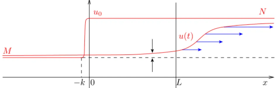
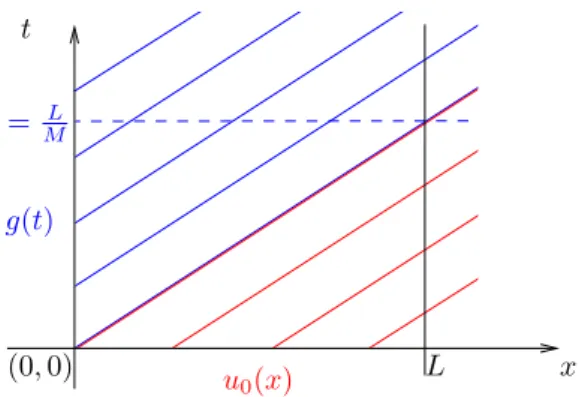
Dans le cas de vitesse M <0, la question du contrôle uniforme se pose également car la condition de Dirichlet homogène sur le bord droit de l'intervalle agit comme un contrôle nul pour le problème des valeurs limites (qui n'a qu'une seule condition aux limites, à x=L ). Ils démontrent un résultat de contrôle uniforme pour T ≥57,2|ML|, ainsi qu'un résultat d'explosion exponentielle plutôt surprenant pour tout T < 2|ML|.
Autour de la m´ethode de Lebeau-Robbiano pour le contrˆole des ´equations para-
In´egalit´es spectrales pour les op´erateurs elliptiques non-autoadjoints et
Dans le cas le moins favorable, où l’on ne dispose que de l’inégalité spectrale (1.29), la construction du contrôle est plus complexe. Cependant, on peut noter que l’inégalité spectrale (1.27) implique, pour les basses fréquences, un coût de contrôle à T−12, lorsque T → 0+.
Analyse et contrˆole d’un mod`ele d’interface diffusive
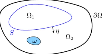
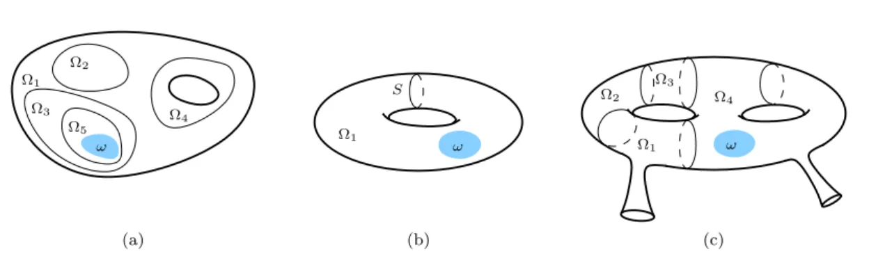
Pour répondre à ces questions, nous montrons l’inégalité de Carleman au voisinage de l’interface S pour l’opérateur Aδ. Pour ce choix de δ, l'inégalité de Carleman (1.41) mesure l'effet tunnel pour le problème d'interface semi-classique.
Contrˆ ole de syst`emes d’´equations hyperboliques, et applications
Stabilisation indirecte de syst`emes d’´equations d’ondes localement coupl´ees 39
Là encore, la méthode permet d'obtenir une estimation de la constante impliquée dans le coût de contrôle de l'équation de Schr¨odinger lorsque T →0+. Contrôle des systèmes d'équations hyperboliques et applications 45 Ce résultat généralise celui de F.
Analyse microlocale de la contrˆolabilit´e de syst`emes de deux ´equations
En particulier, la propriété d'extension unique pour les systèmes en cascade reste valable s'il y a une arête. Enfin, nous avons vu dans la section 1.3.3 que l’étude de la contrôlabilité des systèmes d’ondes couplés nécessite une compréhension des propriétés d’extension uniques des vecteurs propres de l’opérateur elliptique sous-jacent.
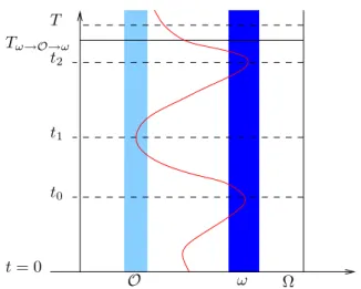
Contrˆ ole uniforme de lois de conservation scalaires dans la limite de viscosit´e
Results in an abstract setting
80 2.4.4 Decay property for the semi-group and construction of the final control 82 2.5 Application to the steerability of parabolically coupled systems. This motivates the explanation of the spectral theory of such operators in section 2.2, following [Agr94]. Russell [Rus73] yields the spectral disparity the controllability of the parabolic system on the related finite-dimensional spectral subspace ΠαH with control costs of the form CeCαθ.
Some applications
However, in the self-adjoint case, the spectral inequalities (2.2) and (2.4) always hold with θ = 1/2, and the controllability result always follows. The null controllability of (2.5) follows from the method described above in cases≤3 (corresponding to θ < 1 in the spectral inequality). In the case n≤2 (corresponding to θ < 1 in the spectral inequality), this estimate is sufficient to restore the null controllability of (2.6).
Spectral theory of perturbated selfadjoint operators
Spectral inequality for perturbated selfadjoint elliptic operators
Inequalities of the type (2.2) were established for the first time in [LR95] for the Laplace operator under a relatively different form. The controllability proof in [LR95] relies on the Hilbert basis property of the eigenfunctions of the Laplace operator. In the subsequent sections, we will consider the additional problem of the abstract parabolic system (2.1) involving A∗ = A0+A∗1.
From the spectral inequality to a parabolic control
From the spectral inequality (2.13), we derive a controllability result for a family of (finite-dimensional) elliptic evolution problems. We then note that point (ii) implies (i) and is itself a direct consequence of expression (2.17), where B∗ is bounded and kGα−1kL(H)≤CeD0αθ from the spectral inequality (2.13). The estimation of the "cost" of control is the key point for the following parabolic properties of fractional controllability.
Lemma 2.19 shows that for any positive T0 (which is set equal to 1 below): for all vk∈PkH there exists erhk (which we know with precision), so that for allw∈Π∗αH,. However, (a Hilbert-appreciated version of) the Paley-Wiener theorem [H¨or83, Theorem 15.1.5] indicates that the inverse Fourier transform of Qk only exists in dual space (G2(R;Y))' of the space of Gevrey functions of order 2. We first note that for T < T the operators ˆe(−iT A) ande−TA A are two isomorphisms of PkH, since the holomorphic functions ˆe(−iT z) ande− T z does not vanish in PKq0 .
Application to the controllability of parabolic coupled systems
Application to the controllability of a fractional order parabolic equation
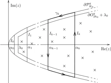
Note that we can replace Aby A+λin (2.1) without changing the controllability properties of the parabolic problem. The idea of proving Theorem 2.7 is to find uniform gaps around the vertical lines Re(z) =αk. Application to the controllability of a parabolic equation of fractional order 89 or equivalently one of the following expressions (see [Haa06]), .
Application to level sets of sums of root functions
The same type of estimates as those performed in the proof of Proposition 2.29 gives the following decay property, for ksufficiently large (k≥Nν), for some constant 0< c <1,. Using arguments from gauge theory given in [Wan08], Theorem 2.36 still holds if we replace the control operatorB in (2.40) by 1EB, for any subset of positive gaugeE⊂(0,T). Under the conditions above, Theorem 2.3 is valid with q = 1/2 and the assumption of Theorem 2.7 is satisfied for p = 2/n.
Appendix
- Properties of the Gevrey function e ∈ G σ , 1 < σ < 2
- A Paley-Wiener-type theorem
- Setting
- Statement of the main results
- Some additional results and remarks
- Notation : semi-classical operators and geometrical setting
We then derive an interpolation inequality and a spectral inequality for the original operator in the spirit of work [LR95]. By the Carleman estimate of Theorem 3.2 we then prove an interpolation inequality of the form presented in [LR95]. More general situations can be handled (interpolation and spectral inequalities, and the null controllability result) due to the local nature of the Carleman estimate of Theorem 3.2.
Well-posedness and asymptotic behavior
Well-posedness
In the sections below we will also use the following tracing formula [LR97, page 486] which links the tangential and volume norms introduced above. Therefore, for all F ∈ H0δ there exists a unique Z ∈D(Aδ) such that AδZ+λZ=F and moreover for a positive constant C we have uniform inδ. A consequence of the properties we have collected about Aδ is the following good theorem for the evolution problem.
As a consequence, we can square the norm H0δ of this equation and integrate at (0, T). Forming the inner product of the first line of this system with ζδ and integrating at (0, T), we get 1. Localization in a neighborhood of the interface 111As a result, we can obtain a convergence result for the control problem under consideration .
Local setting in a neighborhood of the interface
Properties of the weight functions
A system formulation
Conjugation by the weight function
Phase-space regions
Root properties
Microlocalisation operators
Proof of the Carleman estimate in a neighborhood of the interface
Preliminary observations
We now formulate system (3.66) in terms of u•,j in preparation for evaluations in four different microlocal zones. We are now ready to prove various Carleman estimates in four microlocal regions.
Estimate in the region G
On the “r” side, the basic configuration described in Lemma 3.24 (and shown in Figure 3.3) allows us to apply the Calder´on projector technique used in [LR97, LR10]. To obtain estimate (3.77) on the “l” side, we first need a more accurate estimate for the “r” side. The quadratic form Bl is given by Bl(ψ). It remains to estimate the traces on the “l” side from the traces on the “r” side, via the transmission conditions (TC•,j).
Estimate in the region F
Let ˆχ∈C∞(T∗(Rn)) satisfy the same requirements as ˜χ with ˜χ equal to one a neighborhood the support of ˆχ. Since bl−1 does not vanish in a neighborhood of supp( ˆχ), one can set a parametrist for OpT(bl), say OpT(e), withe∈ST1, satisfactorily.
Estimate in the region Z
Since the principal part bl−1 does not vanish in a neighborhood of supp(ˆχ) (see (3.119)), one can introduce a parametric for OpT(bl), say OpT(e), satisfying me∈ST1. Verification of the Carleman estimate in a neighborhood of the interface 129 This equation can be written under the form. Verification of the Carleman estimate in a neighborhood of the interface 131 after using the first relation of (3.124).
Estimate in the region E
On the other hand, replacing E,j in the first equation of (TC•,j) by its expression in the second equation of (TC•,j) gives. 3.147) Here we introduce a class of pseudo-differential operators adapted to the operator Ωδ to perform uniform approximations in the singular limitδ→0+. Proof of the Carleman estimate in a neighborhood of the interface 133 We refer to Appendix 3.8.8 for a proof.
A semi-global Carleman estimate : proof of Theorem 3.2
3.158) To derive the final Carleman estimate, we must sum these microlocal estimates and the many terms in the r.h.s. Note, however, that some powers are critical here, so related terms (in boxes) on the right cannot be "absorbed" directly. In fact, the microlocal region F acts as a buffer: since F is an elliptic region for both Pϕr/l operators, it provides expressions in l.h.s.
Interpolation and spectral inequalities
Interpolation inequality
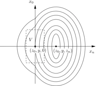
The Carleman estimate of Theorem 3.2 can be applied in an area V close to {z0} ×S× {0} (shown with a dotted line). We also choose α0 such that 0< α0 < α1 must be used for the application of the Carleman estimate of Theorem 3.2. With the geometric context set, we can establish a local interpolation inequality in the vicinity of {z0} ×S× {0}.
Spectral inequality
Far from the interface, the norms Ksδ, s= 0.1 match the usual Hsnorm and similar local interpolation inequalities as (3.163) are proved in [LR95, Lemme 3 page 352]. Now that we have obtained the interpolation inequality (3.163) at the interface, we can apply the procedure described in [LR95, pages 353-356] (smallness propagation) and prove the required global interpolation inequality (3.13).
Derivation of the model
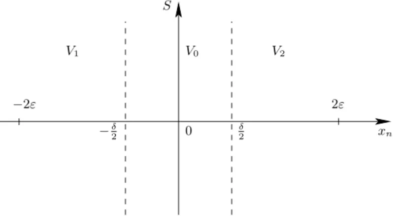
We now want to describe the current three-region model because the thickness δ of the inner region, VO, becomes asymptotically small. Model Derivation 143 This provides a first transmission condition between z1 and z2 that includes the function zs. Yet we show that it cannot be used for modeling the controllability properties of the original system.
Facts on semi-classical operators
In this article, we consider semiclassical operators acting on both variables thex0, x0∈(0, X0) andy∈S. Its kernel is being fixed outside diag (X ×X) in the semi-classical sense: for allχ,χˆ∈C∞ c (X′) such that supp(χ)∩supp( ˆχ) =∅ we have. The first two points of Definition 3.43 actually state that the semiclassical wavefront of the kernel operator is bounded on the conormal bundle of the diagonal of X .
Proofs of some technical results
Noting the proof of Proposition 3.11, we obtain after a local change of variables. In the case µ <0, both imaginary parts of the roots have the same sign, which is the same as the opposite sign of ∂xnϕ. We follow the notation of the proof of Lemma 3.24 above and drop the "r/l" notation here because the same argument holds for both cases.
Introduction
Motivation and general context
Moreover, for internal damping (4.1), the explicit value of the best decay rate κ is given in [Leb96]. Similar questions arise in the analysis of the indirect control of locally coupled parabolic PDEs (see System (4.8) below). In the applications we want to cover (see with p(x) supported locally) this assumption clearly fails.
Results for two coupled wave equations
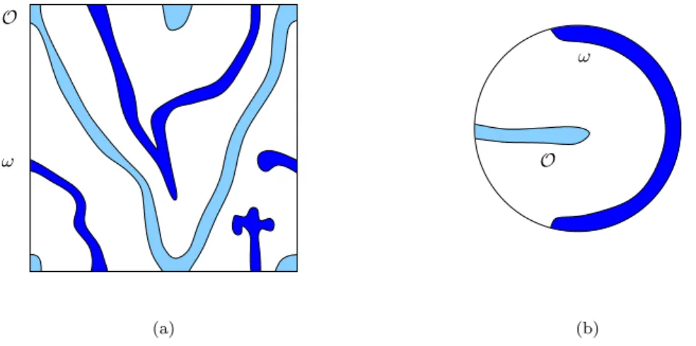
In this paper, the main result concerning the abstract system (4.5) is a polynomial stability theorem under certain assumptions about the operators P and B (see Theorem 4.9 in the restricted case B and Theorem 4.12 in the unbounded case B). However, the interpolation inequality for the associated elliptic problem is unknown in the case ωb∩ωp=∅ and even strong stability is open. Furthermore, this can be a first step to consider first the hyperbolic control problem (4.9) and then its parabolic counterpart (4.8) in the case ωb∩ωp=∅.
Abstract formulation and main results
Abstract setting and well-posedness
Abstract formulation and main results 175 We recall that the energy of this system is given by. Under the assumptions made above, the system (4.12) (and thus (4.5)) is well stated in the sense of semigroup theory. Moreover, the energyE(U) of the solution defined by (4.14) is locally absolutely continuous, and for strong solutions, i.e. when U0∈ D(AP,δ), we have.
Main results
Note that the operator ΠP involved in the estimation of Assumption (A2) is the operator given by Assumption (A1). As one sees in the proof below, δ∗ is very small in Case (i), while in Case (ii), the result holds for a large panel of δ, including the interval (0,1). In this case we are further able to give a simple characterization of the space D(AnP,δ), in terms of the spaces D(An), which is useful in the applications.
Proof of the main results, Theorems 4.9 and 4.12
The stability lemma
This follows from the unbounded nature of the operator B (in the following applications, boundary stabilization). Note also that point (ii) of Theorem 4.9 has no counterpart here since P and B are not of the same nature.
Proof of Theorem 4.9, the case B bounded
Proof of Theorem 4.12, the case B unbounded
Applications
- Internal stabilization of locally coupled wave equations
- Boundary stabilization of locally coupled wave equations
- Internal stabilization of locally coupled plate equations
- Motivation
- Main results
Applying Theorem 4.9, we have proved the following theorem. i) Suppose ωb and ωp satisfy the PMGC. ii). As for coupled waves, we have the following stability result. i) Suppose ωb and ωp satisfy the PMGC. ii). We determine and consider the solutionz of the following elliptic problem ( ∆2z=ψu in Ω,. 4.96). We now look at the multiplierz for (4.72) and evaluate the expression.
Abstract setting
Main results : admissibility, observability and controllability
Some remarks
Two energy levels and two key lemmata
Two energy levels
Two key lemmata
Proof of Theorem 5.10
The coupling Lemma
A first series of estimates
A second series of estimates
End of the proof of Theorem 5.10
From observability to controllability
Applications
Control of wave systems : Proof of Theorem 5.3
Control of diffusive systems
Control of Schr¨odinger systems
Observability for a wave equation with a right hand-side
Preliminary remarks, definitions and notation
Measures, symbols and operators
Some geometric facts
Well-posedness of System (6.4)
Proof of a relaxed observability inequality
End of the proof of Theorem 6.5
Une remarque sur l’obstruction au prolongement unique pour les syst`emes ellip-
Motivation and main results
Some remarks
Structure of the paper, idea of the proofs
Three intermediate propositions
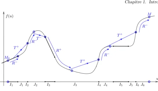
Approximate controllability using a traveling wave
Approximate controllability using a rarefaction wave
Local exact controllability
Proofs of the three theorems
Proof of Theorems 7.1 and 7.2, the convex case
Proof of Theorem 7.3, the non-convex case
Appendix : parabolic regularity estimates
Parabolic regularity estimates for classical solutions