La représentation des systèmes physiques à Port Hamilton est décrite et les changements de coordonnées des systèmes mécaniques sont également résumés. Le problème de la reconstruction de la vitesse des systèmes mécaniques, très pratique, est intensivement étudié dans la littérature.

Notions of stability with respect to input
Input to State Stability(ISS)
In addition, the term β(|x0|,0) can dominate for small t, which serves to quantify the size of the transient (exceeding) behavior as a function of the size of the initial state x0.
Integral Input to State Stability(IISS)
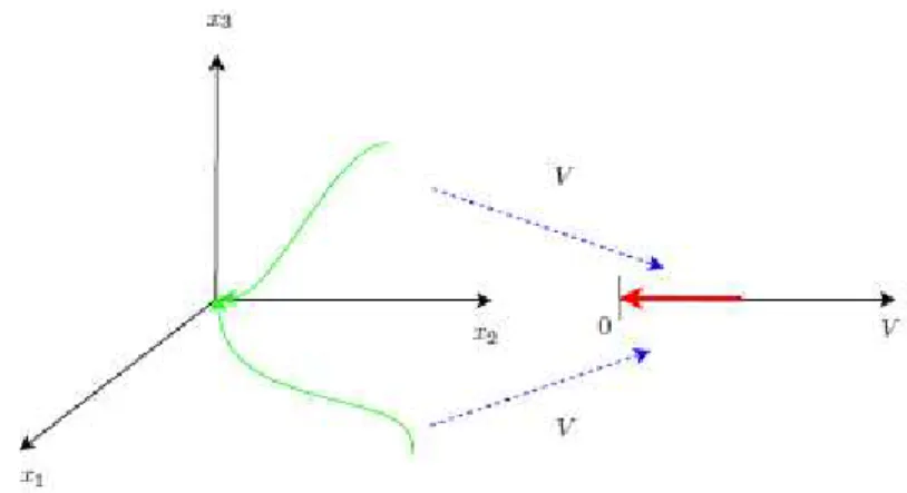
The port–Hamiltonian framework
PREPARATIONS We thus see that the application of Legendre's transformation replaces the system of n second-order differential equations with a set of 2n first-order differential equations with a simple and symmetrical structure. The system (1.7) is called a Port-Controlled Hamiltonian (PCH) system with structure matrix J, dissipation matrix Rand Hamiltonian H.
Immersion and Invariance
Stabilization
In standard or simple mechanical systems, the potential energy is usually a function of the generalized positions V(q) while the kinetic energy is a quadratic function of the velocities (momentums) described as K. The system (1.7) is called the Port-Controlled Hamiltonian System ( PCH) with the structure matrix J, the distribution matrix Rand Hamiltonian H. A4) All trajectories of the system.
Observer design
Necessary and sufficient conditions are provided for the solvability of the problem, in terms of certain rank and controllability properties of the linearized system. One of the central features of passivity-based control (PBC), where the first step is to passivate the system [42], is that the passive output can be easily controlled using integral control (IC) – with random positive gains .
Perturbed port–Hamiltonian systems and problem formulation
Class of systems and control objectives
The purpose of the extra IC is then to ensure that output regulation is robust against external disturbances. This construction is largely inspired by the one proposed in [32], but here we explicitly take into account the presence of the perturbations, which considerably complicates the task. The control objectives are now to maintain the stability of a desired equilibrium and drive a given output towards zero, despite the presence of disturbances.
Notational simplifications
STRETCHED PORT-HAMILTONIAN SYSTEMS AND PROBLEM FORMULATION11 a subtle point that, as explained below, depends on whether the perturbations are. It will be shown below that, for matched perturbations, i.e., those entering the image of g(x) and the passive output, an IC around achieving the objectives. In this chapter we are interested in cases where the disturbance is mismatched and the signal to be adjusted is not the passive output - but is also zero at equilibrium.
Some remarks about equilibria
Robust IC of the passive output
Robustness to matched disturbances
In addition, if y is a detectable output for the closed-loop system, the equilibrium is asymptotically stable. Mbeholds an equilibrium in the closed-loop system, the desired value foru, and consequently for−η, is−d1. The fact that the perturbations in the IC fix the equilibrium value of their state will also be exploited in the case of unmatched perturbations, allowing us to concentrate our attention on the x-components of the equilibrium set.
Discussion and extensions
A feedback equivalence problem
Robust MDICS equivalence guarantees that the control law (2.16) can be implemented without knowledge of the perturbation d2. At this point we make the important observation that in order to solve the robust MDICS equivalence problem, it is necessary to choose the desired value for z3 to be equal to tod2. This, rather arbitrary, choice is made in order to translate MDICS equivalence into an algebraic problem.
Conditions for MDICS equivalence
Global MDICS equivalence
Furthermore, if (2.24) holds, the mapping ˆu(χ) is independent of d2. 2.25) Since∇1ψ(χ) is of integer rank, this equation has a unique solution that defines the mapping ˆ. It is important to note that the disturbance d2, entering through x˙2, is canceled by the termz˙2, which also contains this signal.
Local MDICS equivalence
Of course, there may be other, possibly non-linear, admissible valid maps over a large region of state space. Condition (2.29), on the other hand, is related to the form of the given equilibrium setE. Remembering that the matrices A and E are linearizations of the same vector field at two different points, it is clear that both sets Ecl and Mp play a role in these assumptions.
Robust integral control of a non–passive output
Section 3.8 shows that this is the case for linear systems and nonlinear mechanical systems. In definition 6, the feedback equivalence was said to be robust - for obvious reasons - if the mappings ψ(χ) and ˆu(χ) can be calculated without knowledge of the perturbations2. However, from the dynamics matching equation (2.23) that defines ψ(χ), it is not clear why it would depend on 2.
Examples
Linear systems
Mechanical systems
This fact clearly describes the dynamics of the open-loop system in Euler-Lagrange form. Therefore, the stabilization mechanism is similar to introducing non-linear gyroscopic forces and correspondingly waiting for the potential energy expression. Namely, that the i-th component of the disturbance vector is equal to zero if M(x2) depends on the i-th element of x2, i.e.
Simulation of the classical pendulum system
Conclusions
The stronger property of input-to-state stability, this time with respect to matched and unmatched perturbations, is ensured with the further addition of nonlinear damping. Finally, it is shown that including a partial change of coordinates, the controller can be significantly simplified, preserving input-to-state stability with respect to matched perturbations. Finally, it is shown that including the partial change of coordinates proposed in [48], we obtain a very simple controller that ensures the ISS with respect to matched disturbances.

Problem formulation
Instrumental to our developments is the introduction of coordinate changes, similar to those used in [32] and chapter 2, that preserve the pH structure of the system with the same Hamiltonian function. When M is constant, the dynamics of the system (3.1) in Euler-Lagrange form takes the form. UNMATCHED AND ADJUSTED DISTORTIONS: MECHANICAL SYSTEMS The disturbance d2 thus represents a constant force acting on the system.

Constant inertia matrix
Rejection of constant disturbances
MATRIX OF CONSTANT INERTIA 31 (i) First we take the time derivative of the first equation in (3.5) and substitute it. Second, taking the time derivative z2 in (3.5), we replace ˙p, ˙z2 and ˙z3 with the corresponding equations of state of the open-loop and closed-loop systems. Finally, the last line of the closed loop is given by the integral action of the non-passive output. ii).
ISS for time–varying disturbances
From (3.6) it is clear that, in addition to the addition of the integral action, the Poisson structure of the open-loop system (3.1) is preserved in closed-loop, in the new coordinates. That is, differentiate the first row of (3.10) with respect to time, and replace the derivative of the state by the state equations to obtain the second row of (3.10). Then differentiate the later change of coordinate with respect to time, replace the derivative of the states by the equations of state and solve foru to find the governing law.
Non–constant inertia matrix
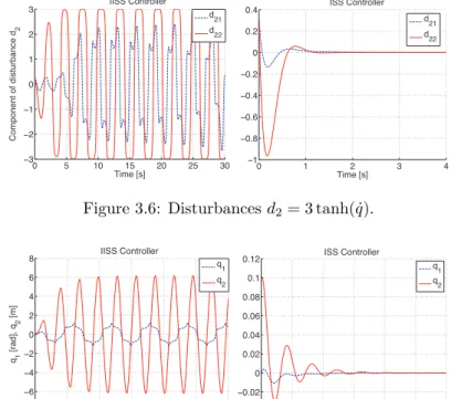
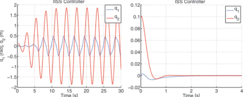
IISS for time–varying matched disturbances
Consider the system (3.1) with constant adjusted perturbation d2 and no unparalleled perturbation, e.g. d1= 0, in closed loop with the control law. i) The closed loop dynamics expressed in the coordinates z1 = q. ii) The desired equilibrium z?:= (q?,0, d2) is asymptotically stable. If the perturbed2 varies with time, it is a closed loop system, which can alternatively be written as. 3.18) is IISS with respect to the input d2(t) with IISS Lyapunov function U¯z(z). Note that the interconnection and damping matrix F(z) of the closed loop pH system is suitably chosen such that the control law does not depend on the unknown perturbation. ii) Considering (3.17) as a candidate Lyapunov function and taking its derivative along the trajectories of the system, it follows.
ISS for time–varying matched and unmatched disturbances
DISTURBANCES AND APPROPRIATE DISTURBANCES: MECHANICAL SYSTEMS disturbances d1(t)end2(t), in closed-loop with the control law. i) The closed-loop dynamics expressed in the coordinates (3.10) takes the perturbed pH form. ii) The closed-loop system is ISS with respect to the input disturbances(d1(t), d2(t)), provided that the Hessian of the potential energy satisfies condition (ii) in Proposition 8. iii). We present (3.12) as candidate ISS Lyapunov function and we calculate its time derivative together with the solutions of (3.21) as follows. A SIMPLIFIED CONTROLLER FOR ADAPTED DISTURBANCES 37Inequality (3.37) and the fact that the function ¯Hz(z) is positive definite and.
A simplified controller for matched disturbances
IISS and GAS for matched disturbances
Note that, as before, the interconnection and damping matrix F(z) of the closed-loop pH system has been suitably chosen so that the control law does not depend on the unknown perturbation. Now from the fact that we have that the system is weakly detectable in the null state from outputz2. If d2 is constant, the closed-loop system can be written as 3.32) If we treat (3.32) as a candidate Lyapunov function and take its derivative along the trajectories of the system, it follows.
ISS for time–varying matched disturbances
UNMATCHED AND MATCHED DISTURBANCES: MECHANICAL SYSTEMS (i) The closed loop dynamics expressed in the coordinates. takes the perturbed pH form. iii). Inequality (3.37) and the fact that the function U(z) is positive definite and radially unbounded guarantees that for any bounded perturbations d2(t), statez(t) will be bounded and the dynamical system (3.36) is ISS . A SIMPLIFIED CHECKER FOR MATCHED DISTURBANCES 41 (iii) Taking d2(t)≡0 in (3.37) and invoking the uniqueness of minimum V yields.
Case study: prismatic robot
It is interesting to note that improved performance is not achieved by injecting larger gains into the loop. On the other hand, the behavior of the IISS controller may not be practically acceptable - as the required forces may exceed the limits of the actuator.
Experiments
Set-up
The desired torque command is then transmitted via TCP/IP to the robot's low-level controller (see Fig. 3.13 for a conceptual representation of the control architecture). To test the performance of the system, we determined the desired link position q∗= q >, where q0=q(0) represents the initial link configuration. To test the robustness of the algorithm, we have numerically perturbed the closed-loop system by adding a constant vector d2 = [2,2]> to the control input u.

Conclusions
This limitation stems from the fact that, in the presence of incommensurable perturbations, a new term involving ˙T appears in the perturbation vector of the transformed system (4.2). Third, and most importantly, since the controller requires a change of coordinates using saturation functions - first introduced in this context in [54] for solving the one degree of freedom case - the irreversibility of these functions. cannot be guaranteed globally and, as clearly shown on page 111 of [40], the claim in [58] is unfounded. Indeed, the claim for the adaptive version of the scheme is unfortunately incorrect, since the argument used to prove the invariance of the estimated domain of attraction S1 is not valid in this case.1 Moreover, the unusual requirement for having the controller initial conditions equal to zero, see Remark 2 in [59], puts a serious question mark on the robustness of the scheme - see also Footnote 2 in Section 4.2.

Main result
Moreover, the controller ensures uniform global asymptotic stability (UGAS) even if the inertia matrix is not bounded from above. Our choice of a pH representation of the mechanical systems stems from the fact that the full-state feedback controller (described in the next section) is a PBC that forms the energy function and assigns a suitable pH structure to the system. The initial conditions of the last component of the controller state, $, are constrained to be positive.
Full–state feedback PBC
A suitable pH representation
This coordinate corresponds to the dynamic scaling factor (shifted) of the I&I observer of [50], which is shown to remain zero bounded for all times. This restriction should be compared with the condition that the controller state must be initialized to zero, imposed in the controller of [59].2.
The PBC and its pH error system
Taking the time derivative of the change of coordinates given in (4.5) and using the control law (4.3) gives the closed loop (4.6), confirming the statement (i). The importance of the PBC presented above depends on the maintenance of the pH structure which is essential for position development. As discussed in [50] and shown in the next section, this assumption is not necessary for the observer's UGEs.
An exponentially convergent momenta observer
To avoid solving the PDE, which may not even exist, an approximate solution is proposed. The ∆q, ∆p mappings play the role of perturbations that are dominated by a dynamic scaling and an appropriate choice of observer dynamics. Imitating [50] choose the dynamics of q|,|p as. where ψ1, ψ2 are some positive state functions defined later. 4.23) In addition, choose the dynamics of the offer.
Proof of proposition 13
Conclusions
Regulation of the non-passive output and rejection of unmatched disturbances is satisfied by adding simple integral action. For varying time perturbations (matched and unmatched), the system is equipped with the IISS and ISS properties.
Future directions
An open question is the robustness of the design to unmodeled, viscous friction in the system. Another challenging problem is the extension of the result to the case of uncertain parameters. The system (A.1) allows the representation of the state space in the coordinates (q,p)7→(q,p) of the form. A.4) with v:=T(q)u a new control signal, a new Hamiltonian function.
Avoiding the gradient on T matrix
Escobar Interconnection and Damping Command, Passivity-Based Control of Port-Controlled Hamiltonian Systems, Automatica pp. Sira-Ramirez, Passivity-Based Control of Euler-Lagrange Systems, Communications and Control Engineering, Springer-Verlag, Berlin, 1998. Dixon, Global adaptive output feedback tracking control of robot manipulators, IEEE Transactions on Automatic Control, Vol.