We also propose simpler scheduling heuristics to compute mappings of the application task graph on the platform. WATERS, and use it to assess and analyze the performance of the three policies through simulations.
Introduction
Section 1.3 presents new algorithms designed to optimize shared cache misses, distributed cache misses, or a combination of both. In Section 1.5 we continue with an experimental evaluation of these algorithms, along with a set of reference algorithms and vendor library routines, on a CPU platform.
Problem statement
Multicore architectures
The shared cache has bandwidth σS, so a block of size S needs a time unit S/σS to be loaded from memory in the shared cache, while each distributed cache has bandwidth σD. Since we assume an ideal cache model with full control over cache behavior, we also assume that the impact of coherence mechanisms on performance can be neglected.
Communication volume
Lower bound on communications
We will first use the previously obtained lower bound to study shared cache misses, and consider everything above this cache level as a single processor and the main memory as a master that sends and receives data. In the case of the distributed cache, we first apply the previous result, on a single core, with cache size CD.
Algorithms
Minimizing shared-cache misses
Load Bc =B[k; j�]in distributed cache Corec LoadCc=C[i�; j�]in distributed cache Corec Compute new contribution: Cc ←Cc+a×Bc Update blockC in shared cache. In order to reduce the number of missed MSs in the shared cache, we extend the maximum reuse algorithm with a new parameter λ.
Minimizing distributed-cache misses
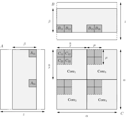
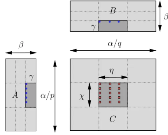
Load elementa=A[k; i�]in the distributed cache of corec Compute the new contribution:Cc ←Cc+a×Bc. Then p×µ elements from a column of Aar accumulate sequentially in the shared cache (pnon contiguous elements are loaded at each step), and then distributed among distributed caches (cores in the same "row" (respectively "column") contributed to the same (or different) element of Abut of different (or the same) p×µfraction of row from B).
Minimizing data access time
Therefore, the communication to computation ratio is β1+µ2, which for large matrices is asymptotically close to β1+�. Load element=A[i�, k�] into corec's distributed cache Compute the new contribution: Cc←Cc+a×Bc.
Performance evaluation through simulation
Simulation setting and cache management policies
SHAREDEQUAL-LRU is the equal-layout algorithm [95] using half of CS (the other half for LRU) Simulated platform In the experiments, we simulated a "realistic" quad-core processor with 8 MB shared cache and four distributed caches of size 256KB dedicated to both data and instruction. We assume that two-thirds of the distributed caches are dedicated to data, and one-third to the instructions.
Cache management policies: LRU vs. ideal
Results using a more pessimistic distribution of half for data and half for instructions are also given. An LRU setting based on the LRU cache data replacement policy, but reporting only half of the cache size to the algorithm.
Performance results
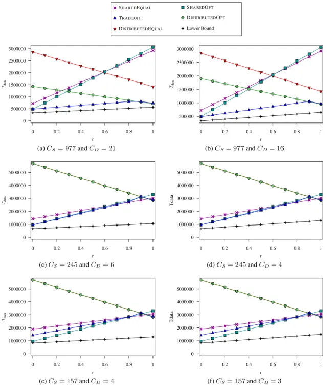
This is confirmed by Figure 1.10band1.10d, in which we see that TRADEOFF and SHAREDOPT are associated with the IDEAL setting. This is confirmed by Figure 1.11 band 1.11d, in which we see that SHAREDOPT significantly outperforms TRADEOFFE and using the IDEAL setting.

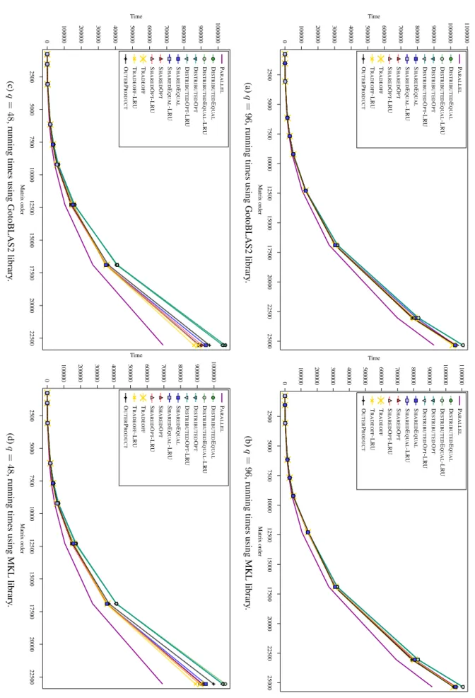
Performance evaluation on CPU
Experimental setting
DISTRIBUTEDOPT-LRU is DISTRIBUTEDMMRA using half of CD (other half for LRU) – TRADEOFF is TRADEOFFMMRA using all CS and CD. TRADEOFF-LRU is TRADEOFFMMRA using half of CSandCD (other half for LRU) – DISTRIBUTEDEQUAL is the equal representation algorithm [95] using the whole CD.
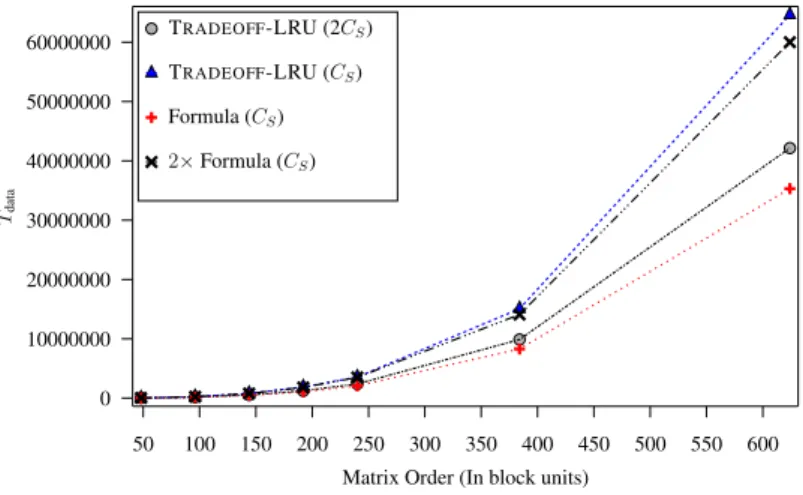
Performance results: execution time
The equal-layout algorithm is derived from four versions: shared/distributed version, and ideal/LRUcache. SHAREDOPT-LRU is SHAREDMMRA that uses half of WK, and the other half is used as a buffer for LRU policy.
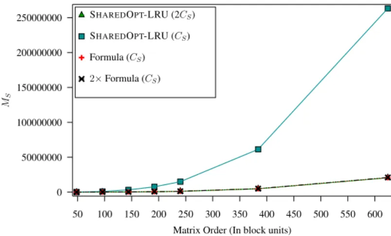
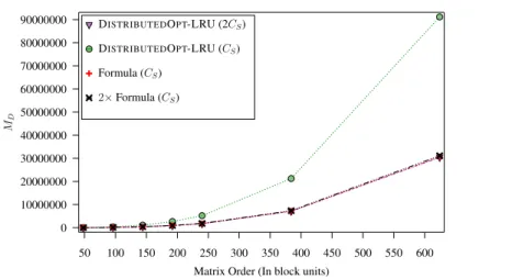
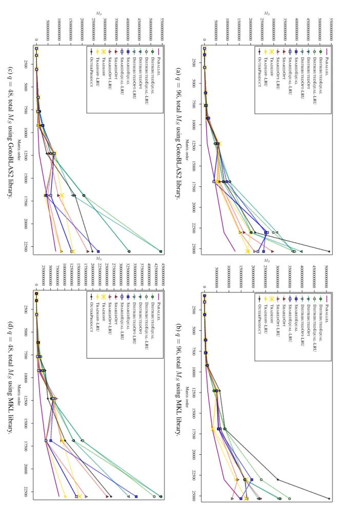
Performance results: cache misses
In conclusion, cache misses do not appear to have a significant impact on runtimes (but MS appears to be more important than MD, as expected). Note that the lower associativity of CD again here has a greater impact on casmises and significantly increases the MD.
Performance evaluation on GPU
- Experimental setting
- Adaptation of MMRA to the GT200 Architecture
- Performance results: execution time
- Performance results: cache misses
To deal with rectangular tiling, let η be the number of columns of the block in CD, and χ its counterpart for the number of rows. The following experiment evaluates the number of shared cache misses recorded by each algorithm.
Conclusion
The QR factorization of anm-by-n matrix with n ≤ m is used to compute the orthogonal basis (Q factor) of the column span of the initial matrix A. The focus of this chapter is on improving the overall degree of parallelism of the algorithm.

The QR factorization algorithm
Kernels
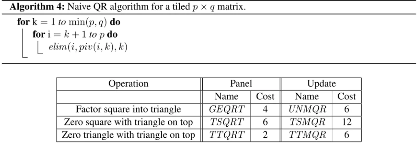
In this table, the unit of time is the time to perform n33b floating point operations. Note that TSQRT(i, piv(i, k), k) and UNMQR(piv(i, k), k, j) can be performed in parallel, as well as UNMQR operations on different columns j, j� > k.
Elimination lists
From an algorithmic perspective, TT kernels are more attractive than TSkernels, as they offer more parallelism. The transition from the aTSkernel algorithm to the aTT kernel algorithm is done implicitly by Hadri et al.
Execution schemes
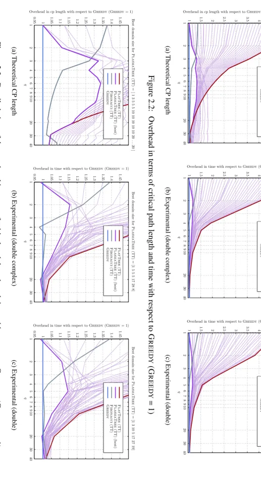
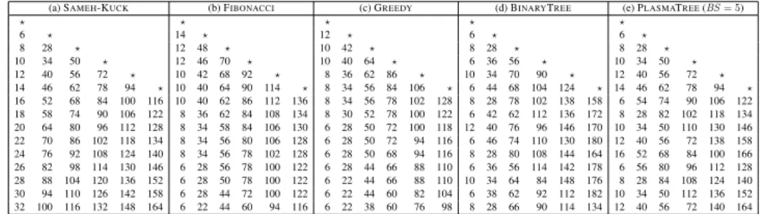
Critical paths
Coarse-grain algorithms
In particular, the proportional letterpandqbe,p=λq, with a constantλ >1: FIBONACCI is asymptotically optimal, because the axis is of order √q, therefore its critical path is 2q+o(q). For q×q square matrices, the critical paths are slightly different (2q -3 for SAMEH-KUCK, x+ 2q -4 for FIBONACCI), but the important result is that all three algorithms are asymptotically optimal in that case.
Tiled algorithms
In the coarse-grained model, ALG ends the first column in the timex, so the critical path of its slowed version is 6x+ 22(q−1). In the quadratic case, we see that the critical path length of distributed algorithms is typically inO(nn2b).
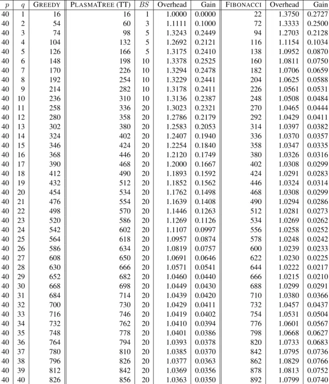
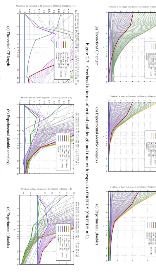
Experimental results
For each experiment, we provide a comparison of theoretical performance with actual performance. As more columns are added, the parallelism of the algorithm increases and the critical path becomes less of a limiting factor, so that the performance of the cores comes to the fore.

Conclusion
DataCutter-Lite [48] is a modification of the DataCutter framework for the Cell processor, but it is limited to simple streaming applications described as linear chains, and thus cannot handle complex task graphs. StreamIt [47,91] is a language developed to model streaming applications; a version of the Streamit compiler has been developed for the Cell processor, but it does not allow the user to specify the mapping of the application and thus precisely control the application.
General framework and context
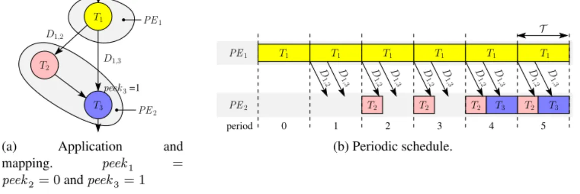
The application consists of a single task graph, but all flow data sets must be processed according to this task graph. Consider processing the first set of data (eg, the first image of a video stream) for the application depicted in Figure 3.1b.

Adaptation of the scheduling framework to the QS 22 architecture
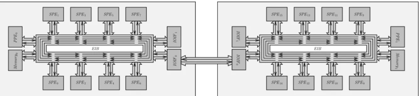
Platform description and model
The output capacity of the processing elements and the main memory is also limited to 25 GB/s. When an SPE ofCell0 reads from a local memory inCell1, the transfer bandwidth is at 4.91 GB/s.
Mapping a streaming application on the Cell
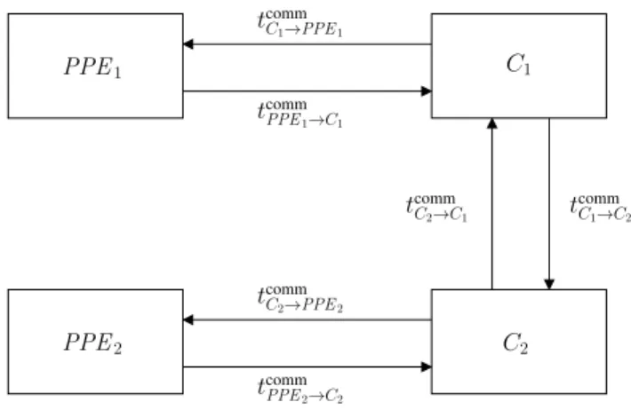
It must send the result Dk,l of the previous instance to the processing element responsible for each subsequent task Tl. Finally, it must retrieve the dataDj,k of the next instance from the processing element assigned to each predecessor taskTj.
Optimal mapping through mixed linear programming
So the size of the buffer needed to store this data is tempk,l = datak,l×(firstPeriod(Tl)−firstPeriod(Tk)). The size of the linear program depends on the size of the task graphs: it counts n|VA|+n2|EA|+ 1 variables.
Low-complexity heuristics
- Communication-unaware load-balancing heuristic
- Prerequisites for communication-aware heuristics
- Clustering and mapping
- Iterative refinement using D ELEGATE
Tk∈SwP P E(Tk)in the case of a PPE where the set of tasks is mapped onto the processing element. If it is a set of SPEs, the procedure CELLGREEDYSET is used to check memory constraints and calculate the new processing time.
Experimental validation
Scheduling software
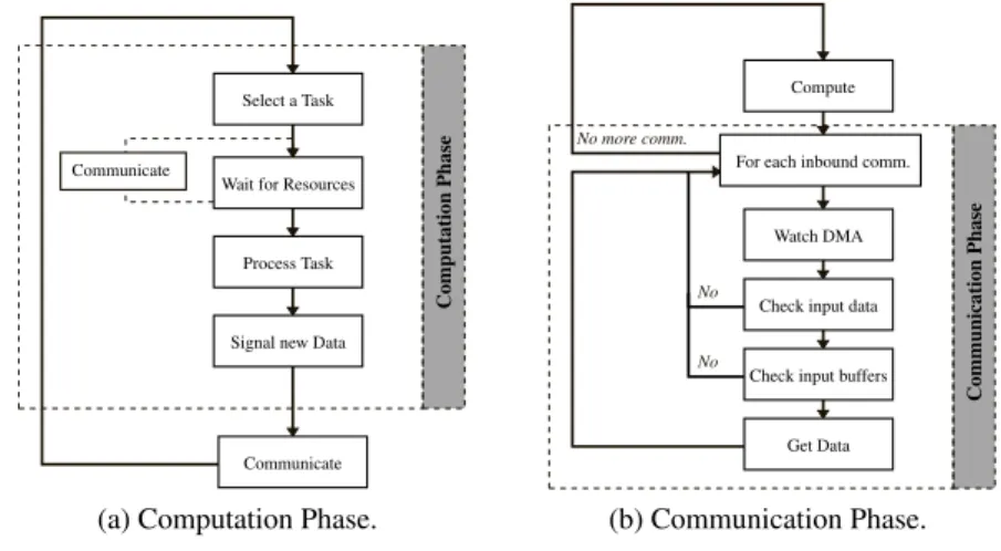
If all required resources are available, the selected job is processed, otherwise it goes to the communication phase. Each thread then internally chooses the next function (or task graph node) to run on the specified schedule.
Application scenarios
Experimental results
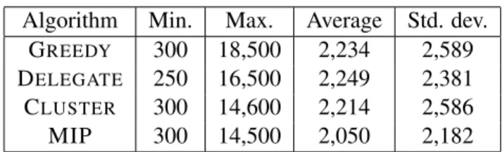
The average throughput of DELEGATE is very close to the throughput of MIP (greater for small task graphs, but smaller for large task graphs), and GREEDY achieves about 90% of the throughput of the MIP. Figure 3.13a shows the evolution of the ratio between the experimental throughput of MIP and the predicted throughput as a function of the CCR.
Related Work
To our knowledge, none of the existing frameworks targeting the Cell processor make it possible to implement our static scheduling strategies. However, these studies usually consider a single DAG and try to minimize the completion time of this DAG, while we consider a piped version of the problem, when several instances of a shared DAG need to be processed.
Conclusion
The nodes of the tree correspond to tasks, and the edges correspond to dependencies between tasks. MINIO Given the sizeM of main memory, determine the minimum I/O volume required to execute the tree.
Background and Related Work
Elimination tree and the multifrontal method
We address the MINMEMORY problem in Section 4.4, present complexity results for mail-order traversals, and present the exact MinMem algorithm. We then consider the MINIO problem in Section 4.5, assess the NP hardness of this problem, and design heuristics.
Pebble game and its variants
The join can be restricted so that two nodes of the elimination tree are joined only if the corresponding L-factor columns have the same structure below the diagonal [36].
Models and Problems
- Application model
- In-core traversals and the M IN M EMORY problem
- Model variants
- Out-of-core traversals and the M IN IO problem
Input: treeT withpnodes, available memoryM, orderingσof the nodes Output: whether the traversal is feasible. The order of the I/O operations is done through a second functionτ so that τ(i) is the step in which to move the input file from taski(of sizefi) to secondary memory (τ(i) = ∞ means that this file is never moved to secondary memory).
The M IN M EMORY Problem
Postorder traversals
We now define the MINIO problem, which requires traversal outside the core with the minimum amount of I/O volume. Given a treeT and a fixed amount of main memoryM, determine the smallest I/O extentIO required by the solution OUTOFCORETRAVERSAL(T, M).
The Explore and MinMem algorithms
When no more nodes can be improved to the cut (which is easily tested using their respective memory peak), then the algorithm outputs the current cut. To estimate the complexity of the MINMEMORY problem, we consider the moment when each node is first visited by Explore, that is, for each node, the first call to onExplore(T, i).
The M IN IO Problem
NP-completeness
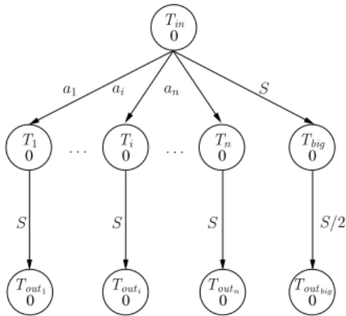
Altogether, the overall complexity of the algorithm is O(p2). ii) determine the minimum input/output volume needed for each pass after ordering the tree, (iii) determine the minimum input/output volume needed for each tree pass. Now for (i), get any ordering of nodesσ that executes Tbig immediately after the root taskTin.
Heuristics
Experiments
- Setup
- The Data Set
- Results for M IN M EMORY
- Results for M IN IO
- More on PostOrder Performance
The first objective is to evaluate the performance of PostOrder in relation to the memory requirement of the resulting traversal relative to the optimal value. The goal is to further assess the performance of PostOrder in relation to the resulting memory requirement.

Conclusion
For the MINMEMORY problem, we proposed an exact algorithm that works faster than Liu's reference alternative [69]. We have shown that the MINIO problem is NP-complete, as are some of its variations (for example, we have shown that finding the mail-order traversal that minimizes I/O volume is NP-complete).
Introduction
The first of these, PARALLEL, still uses the same number of X+Y tape drives, and therefore suffers from the same problem of reducing the serviceability of the system and increasing the start-up time. The simulation setup is provided in Section 5.6, as well as the results of the comprehensive simulations.
Related work
We first briefly review related work in Section 5.2 and describe the framework in Section 5.3.
Framework
Platform model
Each shifter node has 24 cores and 96 GB of RAM; the movement mode is associated with 10 tape units.
Problem statement
Tape archival policies
RAIT
These EC blocks are calculated in memory before data blocks are actually written to tapes. The behavior of RAIT is shown in Figure 5-1: when all tapes are empty, the first X blocks are written to tape drives TD1 to TDX, while the Y EC blocks are written to TDX+1 to TDX+Y.
PARALLEL
However, it may happen that some (or all) tapes dedicated to storing EC blocks fill up before the data tapes (as depicted in Figure 5.2a), EC blocks are generally less compressible. Because of the hardware compression mechanism embedded in tape drives, and given that EC blocks are generally less compressible than data blocks, tape occupancy is slightly unbalanced.
VERTICAL
Data is contiguous on tape and EC blocks do not need to be read when data is read. Like the PARALLEL policy, EC blocks are written on dedicated tapes, which means that tape occupancy can be less balanced than with RAIT. ii) although the whole system may be able to handle more requests simultaneously, each request will take more time to complete as there is no data parallelism with VERTICAL. iii) the tape drive is not available for application I/O when the EC blocks are written.
Scheduling archival requests
The role of the MAX-LIGHTLOAD system parameter is to adjust the process load threshold. If then idle tape drives that can host a process still remain, a new process is created that matches the type of the busiest queue.
Performance evaluation
Experimental framework
A new file is created 90% of the time if the request is a write operation, otherwise the existing file is rewritten. Each request is provided with an X+Y resistance scheme randomly selected from a set of representative schemes.
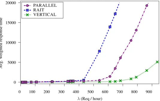
Results with a single policy
The underlying objective of this experiment is therefore to determine the impact of this pitfall on the weighted mean response time. The next experiment focuses on evaluating the impact of the load balancing period MINLBINTERVAL on the average weighted response time.
Results with multiple policies
Conclusion
We conducted an extensive series of experiments to assess the performance of the three archiving policies. In IPDPS'09: Proceedings of Workshops of the 23rd IEEE International Parallel and Distributed Processing Symposium.