HAL Id: hal-01009235
https://hal.archives-ouvertes.fr/hal-01009235
Submitted on 17 Jun 2014
HAL is a multi-disciplinary open access archive for the deposit and dissemination of sci- entific research documents, whether they are pub- lished or not. The documents may come from teaching and research institutions in France or abroad, or from public or private research centers.
L’archive ouverte pluridisciplinaire HAL, est destinée au dépôt et à la diffusion de documents scientifiques de niveau recherche, publiés ou non, émanant des établissements d’enseignement et de recherche français ou étrangers, des laboratoires publics ou privés.
A simplified approach for the calculation of acoustic emission in the case of friction-induced noise and
vibration
Kevin Soobbarayen, Sébastien Besset, Jean-Jacques Sinou
To cite this version:
Kevin Soobbarayen, Sébastien Besset, Jean-Jacques Sinou. A simplified approach for the calculation of acoustic emission in the case of friction-induced noise and vibration. Mechanical Systems and Signal Processing, Elsevier, 2015, 50-51, pp.732-756. �10.1016/j.ymssp.2014.05.014�. �hal-01009235�
A simplified approach for the calculation of acoustic emission in the case of friction-induced noise and
vibration
K. Soobbarayen1,a , S. Besset1,b, and J-.J. Sinou1,c
1Laboratoire de Tribologie et Dynamique des Syst`emes, UMR CNRS 5513, Ecole Centrale de Lyon, 36 avenue Guy de Collongue 69134 Ecully Cedex, France
{akevin.soobbarayen, bsebastien.besset,cjean-jacques.sinou}@ec-lyon.fr
Abstract
The acoustic response associated with squeal noise radiations is a hard issue due to the need to consider non-linearities of contact and friction, to solve the associated nonlinear dynamic problem and to calculate the noise emissions due to self-excited vibrations. In this work, the focus is on the calculation of the sound pressure in free space generated during squeal events.
The calculation of the sound pressure can be performed by the Boundary Element Method (BEM). The inputs of this method are a boundary element model, a field of nor- mal velocity characterized by a unique frequency. However, the field of velocity associated with friction-induced vibrations is composed of several harmonic components. So, the BEM equation has to be solved for each frequencies and in most cases, the number of harmonic component is significant. Therefore, the computation time can be prohibitive.
The reduction of the number of harmonic component is a key point for the quick estima- tion of the squeal noise. The proposed approach is based on the detection and the selection of the predominant harmonic components in the mean square velocity. It is applied on two cases of squeal and allows us to consider only few frequencies.
In this study, a new method will be proposed in order to quickly well estimate the noise emission in free space. This approach will be based on an approximated acoustic power of brake system which is assumed to be a punctual source, an interpolated directivity and the decrease of the acoustic power levels.
This method is applied on two classical cases of squeal with one and two unstable modes.
It allows us to well reconstruct the acoustic power levels map. Several error estimators are introduced and show that the reconstructed field is close to the reference calculated with a complete BEM.
1 Introduction
The brake squeal phenomenon is characterized by high frequency noise emissions due to friction- induced self-excited vibrations. The prediction and the calculation of squeal noise are complex tasks which are composed of several steps [1]. The first one deals with the nonlinear modeling with the definition of the mechanical system geometry, the introduction of nonlinear laws corre- sponding to the contact and friction phenomenon over the interface. Then, a stability analysis is performed with respect to one or several parameters. This analysis allows us to detect the unstable equilibrium configurations that may lead to squeal and provides the fundamental fre- quencies of the unstable modes. The next step consists of calculating the time responses and it has been shown in the literature that the stationary regime associated with the squeal has a spectrum composed of fundamental frequencies (that should be different from the frequencies of
the unstable modes [2]), their harmonic components and also their linear combinations. Then, the calculation of the noise radiations during squeal event can be performed with the Boundary Element Method [3, 4]. This is the classical way to well estimate the sound pressure. This nu- merical method is based on the resolution of the Kirchhoff-Helmholtz equation which depends on the wave frequency. Therefore, the sound pressure calculation has to be carried out for each harmonic component of the velocity field.
In this aim, the multi-frequency acoustic calculation method has previously been developed [1]. The method is based on the decomposition of the velocity into Fourier series. Therefore, the global wave is decomposed into elementary waves with a unique frequency. The BEM is then applied for each wave and the global sound pressure field is calculated by superposition.
The application of the BEM is composed of three steps. Firstly the boundary element model is built and it is composed of the system skin. Secondly, the surface sound pressure is calculated and finally, the sound pressure in the free space is evaluated by using the surface pressure.
So, the latter is calculated for each frequency and the free field pressure is calculated for each frequency and each field plane. However, the number of frequencies can be significant making the computation time prohibitive.
In a previous work [1], it has been shown that only few harmonic components are predom- inant in the acoustic response. So it can be useful to determine these frequencies before the application of the multi-frequency acoustic calculation method. The first aim of the current paper is to develop a criterion based on the mean square velocity convergence (i.e. the dynamic response) which allows us to detect the predominant frequencies.
The second objective of this work is to propose a new method which allows to quickly well estimate the sound pressure in the free field. In order to calculate the radiations, the directivity and a propagation model which describe the level decrease are required. The main idea is to determine the directivity with the BEM and to determine an analytical function with an interpolation. Finally, for each frequencies, the sound pressure can be evaluated at every field points without the BEM.
The present paper is organized as follows. Firstly, the vibroacoustic of a squealing disc brake system is presented. The brake system under study is detailed and the dynamic and acoustic responses for two cases with one and two unstable modes are given. Secondly, the criterion which allows us to detect the predominant frequencies in the dynamic response is presented and applied for the two cases under study. Thirdly, the acoustic approximation method is presented and several sound pressure error estimators are presented. Finally, the acoustic method is applied and validated on the two cases.
2 Vibroacoustic of a squealing brake system
In this section, the simplified disc brake model under study is presented. The finite element model, the modeling of the frictional interface and the stability results are detailed. Next, the focus will be on the time responses associated with two classical cases of squeal with one and two unstable modes. Finally, the multi-frequency acoustic calculation method is applied to calculate the surface sound pressure and the sound pressure radiated in free space.
2.1 Brake system modeling
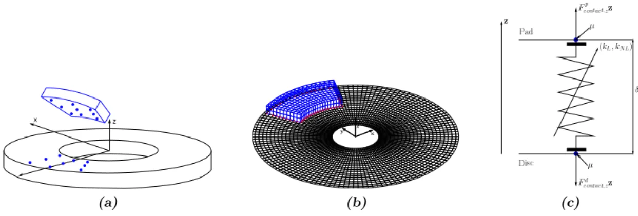
The two main components involved in the squeal are the disc and the pad which share a frictional interface. This allows to focus on a simplified disc brake system composed of a circular disc and a pad as illustrated in Figure 1. The inner radius of the disc is clamped due to the shaft connection and the outline of the upper surface of the pad can only translate along the normal
(a)
x z y
(b) (c)
Figure 1: Brake system model and boundary element model. (a): Simplified disc brake system and selected contact nodes•; (b): boundary element mesh used for the acoustic calculation.
z−direction to represent the caliper connection. In this work, automotive brake dimensions have been used.
Contact and friction phenomenon occurs over the common frictional interface which is mod- eled with nine uniformly spaced contact points as illustrated in Figure 1 (a).These contact elements are arbitrarily chosen and these number and positions strongly influence the stability analysis. However, increasing the number provides a better description of the interface but the calculation performances can be much reduced. In this study, nine elements seem to be a good compromise [2].
Between the previous selected points, nonlinear contact and friction forces are introduced.
The nonlinear contact force vector is described with linear and nonlinear stiffnesses and con- tact/loss of contact configurations is considered. The cubic contact law associated with nonlinear contact elements takes the following expression:
Fcontact,zd =
( kLδ+kNLδ3 ifδ <0
0 otherwise (1)
where δ =Xp−Xd is the relative displacement,Xp and Xd denote the normal displacements of the pad and the disc respectively. kL and kNL are the linear and cubic stiffnesses, Fcontact,zp andFcontact,zd are the components of the normal contact force vector applied to the pad and the disc respectively. It can be noted that Fcontact,zp = −Fcontact,zd . This contact force expression has been chosen to fit experiments as explained in [5]. The main limitation of this formulation is that it allows penetration between the disc and the pad due to the fact that the contact stiffnesses are constant. A penalty algorithm which adjusts these stiffnesses can be used to apply an impenetrability condition.
Involving friction, the friction coefficientµis assumed to be constant for the sake of simplicity and the classical Coulomb’s law is used to model the friction over the interface. Thus, the nonlinear friction force vector over the frictional interface plane is defined by:
Fdfriction = µFcontact,zd vr
||vr||
Fpfriction = −Fdfriction
(2)
whereFdfriction andFdfriction are the friction force vectors applied to the disc and the pad respec- tively. vr is the sliding velocity between the disc and the pad. A permanent sliding state is considered. Finally, the braking pressure which activates the contact between the disc and the pad is modeled with a constant uniform pressure applied over the back-plate of the pad.
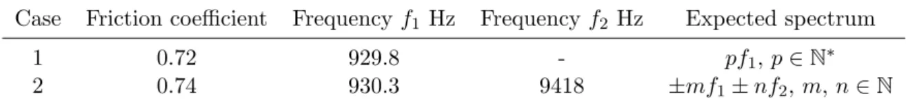
Case Friction coefficient Frequency f1 Hz Frequencyf2 Hz Expected spectrum
1 0.72 929.8 - pf1,p∈N∗
2 0.74 930.3 9418 ±mf1±nf2,m,n∈N
Table 1: List of cases under study. (1): One unstable mode; (2): two unstable modes.
This simplified modeling does not attempt to capture all the nonlinear effects but is suitable for mode coupling instabilities. Moreover, it serves to illustrate the simplified approach for the calculation of acoustic emission in the case of friction-induced noise and vibration.
A Craig and Bampton reduction method [6] is used to reduce the system size. The reduction basis is composed of all the attachment modes and the first hundred eigenmodes of the structure assuming the interface nodes are held fixed. This reduction provides a good correlation between the whole and the reduced brake models until 20 kHz which is sufficient for the frequency range of interest of the present study.
Finally, the equations of motion in the reduction space are given by Eq. 3:
M ¨X+C ˙X+KX=FNL(X) +F (3)
whereM,CandKare mass, damping and stiffness matrices. Xis the generalized displacement vector and the dot denotes derivative with respect to the time. FNL defines the global nonlinear force vector which contains linear and nonlinear parts of the contact force vector and also the friction force vector applied to the disc and the pad. The vector Fcorresponds to the braking pressure applied over the pad back-plate. Involving the damping matrixC, the following modal damping is considered: a damping percentageξ is used for stable modes and a damping rate ζi
for theith coalescent modes, as explained in [1].
For the interested reader, extensive reviews about the modeling of the automotive disc brake squeal can be found in [7, 8].
2.2 Stability analysis
The stability can now be estimated by analyzing the eigenvalues of the linearized equation of motion. The linearization is performed near the sliding equilibrium configurationXsliding which corresponds to the quasi-static configuration of the rotating brake system under the braking pressure. The eigenvalues and the eigenvectors of the linearized system are given by the following equation:
λ2M+λC+ (K−JNL,Xsliding)
Φ=0 (4)
whereλis the diagonal matrix which contains the eigenvalues,Φdenotes the eigenvector matrix, and JNL,Xsliding is the Jacobian of the nonlinear force vector. The eigenvalues are complex due to friction and if all the eigenvalues have a negative real part, the sliding equilibrium is stable and the system reaches the sliding equilibrium configurationXsliding. If at least one real part is positive, then the sliding equilibrium is unstable, the system diverges and self-excited vibrations are generated. In this work, this analysis is carried out with respect to the friction coefficient µ. By analyzing the eigenvalues with respect to µ, two instabilities with one and two unstable modes are detected. The two cases under study in this work are listed in Table 1.
The stability analysis, based on the associated linear system, allows to predict the squeal onset and this ability has been experimentally validated by Massi et al. [9]. However, the authors highlight the fact that a nonlinear model needs to be used to reproduce the squeal in the time
domain. That is why a full time integration of the nonlinear system has to be performed to calculate the nonlinear friction-induced squeal vibrations.
2.3 Self-excited vibrations
The time responses are calculated with a Runge-Kutta integration scheme for the cases 1 and 2. The initial conditions correspond to the associated sliding equilibrium configurations with a slight disturbance. The results are similar with those shown in [1] and in order to condense the contents of the present paper, only the spectrum of the stationary regimes for the two cases is given.
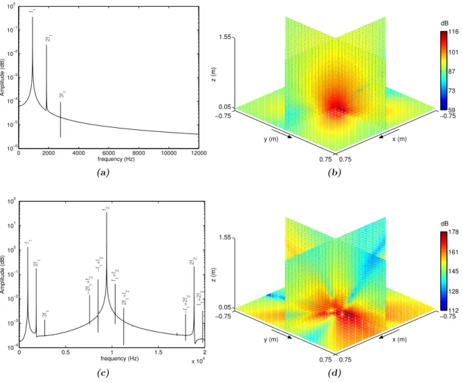
For the case 1, Figure 2 (a) indicates that the harmonic components are composed of the fundamental frequency f1 and several harmonic as 2f1 and 3f1.
The case 2 presents a more complex spectrum composed of the fundamental frequencies f1 and f2, several harmonic components 2f1, 3f1, 2f2, and also their linear combinations of the form: ±mf1±nf2 wherem andn are positive integers (see Figure 2 (b)).
These dynamics responses strongly depend on the contact status due to successive activa- tion/deactivation of the contact stiffnesses during contact/loss of contact configurations. The interface motion is therefore complex and the interested reader could find more details about the contact status during squeal event in [2].
2.4 Noise emissions
The numerical study of acoustic radiations due to squeal events is a recent topic. In 2004, an approach using a semi analytical plate kinematic has been used to estimate the noise radiations due to modal force vibrations [10]. More recently, Oberst et al. [11] propose complete guidelines for the numerical acoustic investigation of squeal. This study highlights the fact that the pad geometry, the interface refinement and the contact/friction formulation have a strong impact on the noise radiations in terms of both the levels and the directivity. The two mentioned papers focus on the radiations generated with a forced dynamic response for a unique frequency. With this method, it is possible to well estimate the radiations associated with a given mode. In the present paper, the proposed approach involves the global radiations generated by the whole dynamic responses i.e. with the whole nonlinear spectrum for a simplified phenomenological brake model.
For this acoustic study, the boundary element model is composed of the upper part of the system skin as illustrated in Figure 1 (b). Actually, it is assumed that these surface radiations lead the outside global noise radiations. Moreover, over the connected points between the disc and the pad (i.e. the red points in Figure 1 (a)), the normal velocities are averaged. Then the multi-frequency acoustic calculation method allows us to estimate the noise levels over the mesh and at every points in free space. The main idea of this approach is to apply the BEM for each frequency and to calculate the global sound pressure by superposition. This method has been developed in a previous work and the interested reader could refer to [1]. The BEM contains two main steps: firstly the surface sound pressure calculation PωS which depends on the surface normal velocity field ˙Xn, then the free space sound pressure Pω is calculated with the surface sound pressure. For more details about the Boundary Element Method, the reader could refer to [3, 4]. The previous fields depend on the wave frequencyω, that is why the BEM has to be applied for each harmonic component. The global sound pressure field is calculated by superposition and will be denoted byPin the free space andPS over the mesh. For the two cases under study, the focus will be on the sound pressure levels Lp,bem = 10 log10(PP∗/Pref2 ), wherePref = 20µPa and the star denotes the conjugated.
0 2000 4000 6000 8000 10000 12000 10−6
10−5 10−4 10−3 10−2 10−1 100
frequency (Hz)
Amplitude (dB) f1 2f1 3f1
(a)
−0.75
0.75
−0.75
0.75 0.05
1.55
x (m) y (m)
z (m)
59 73 87 101 116 dB
(b)
0 0.5 1 1.5 2
x 104 10−4
10−3 10−2 10−1 100 101 102
frequency (Hz)
Amplitude (dB) f1 2f1 3f1 −2f1+f2 −f1+f2 f2 f1+f2 2f1+f2 −f1+2f2 2f2 f1+2f2
(c)
−0.75
0.75
−0.75
0.75 0.05
1.55
x (m) y (m)
z (m)
112 128 145 161 178 dB
(d)
Figure 2: Nonlinear spectra and sound pressure levels in free space for the cases 1 and 2. (a):
Spectrum case 1; (b): Lp,bem case 1; (c): spectrum case 2; (d): Lp,bem case 2.
For the case 1, the total sound pressure levels radiated in free space are composed of one main lobe along thez-direction, but four lobes are present over the (x,y) plane as indicated in Figure 2 (c).
For the case 2, the free space radiations are more complex with several main directions of propagation as illustrated in Figure 2 (d). This is due to the contribution of two unstable modes in the dynamic response. Moreover, noise levels are also higher than for the case 1 due to the higher amplitude of velocity.
It can be concluded that both the dynamic and acoustic responses are much complex for the multi-instability case: the directivity presents several main propagation directions and higher noise levels. The computation time of the surface pressure can be prohibitive due to the mesh refinement and the frequency dependency. However, it can be noticed that the total surface pressure is widely led by only few harmonic components. This feature has been investigated in details in [1] where a convergence study of the sound pressure is carried out with respect to the number of retained harmonic components. Therefore, if a criterion can be determined to select the predominant harmonic components before solving the acoustic problem, it will be possible
to quickly well estimate the sound pressure.
These numerical results are not experimentally confirmed but the main objective of the present study is to propose a harmonic components selection method and an acoustic approx- imation method. So, the development and the validation of the proposed simplified approach are valid. However, squeal events with one or two unstable modes at the same time have been experimentally reported in [12, 13] respectively.
3 Harmonic components selection method
As explained in the previous section, the dynamic response associated with the squeal is com- posed of several frequencies. These harmonic components can be numerous as for the case with two unstable modes and the sound pressure has to be calculated for each frequency. However, as previously explained, the total radiation is mainly led by few harmonic components. In this section, a criterion which allows the detection of the predominant frequencies is presented. The main idea is to select the harmonic components which “significantly” contribute to the mean square surface normal velocity. By this way, an optimal Fourier basis is built with a limited number of harmonic components.
3.1 Mean square velocity convergence
The initial Fourier basis is composed of all the detected harmonic components sorted by increas- ing order. The detected components are linear combinations of the fundamental frequencies and are of the form:
k1w1+k2w2+...+kiwi+...+kpwp (5) withki∈ [−Nh,Nh],Nh is the highest order andpdenotes the number of detected fundamen- tal frequencies. Fourier transform of the surface normal velocity field provides the following expression:
X˙n(t)≈
Nh
X
k1=−Nh
...
Nh
X
kp=−Nh
ak1, ..., kpcos(k1w1+...+kpwp)t+bk1, ..., kpsin(k1w1+...+kpwp)t (6) where ak1, ..., kp and bk1, ..., kp are the Fourier coefficient vectors corresponding to the linear combination of w1, ..., wp. By introducing the basisω =[w1 ... wp]T and the vector τ =ωt, the approximated velocity takes the following form:
X˙n(τ)≈a0+ X
k∈Zp
akcos(k.τ) +bksin(k.τ) (7) where the vector k contains the coefficients of all the linear combinations of the fundamental pulsations ωj. It can be noticed that the velocity associated with the harmonic component m is of the following form:
X˙n,m(τ) =akmcos(km.τ) +bkmsin(km.τ) (8) The mean square velocity associated with a truncation N and denoted by Ek,N can now be calculated:
Ek,N = v u u t 1
Ndof
"
a0+
N
X
m=1
X˙n,m(τ)
#T"
a0+
N
X
m=1
X˙n,m(τ)
#
(9)
where N denotes the current truncation and Ndof is the number of degree of freedom of the acoustic model. Then, the mean square velocity associated with the global responseEk,ref can be calculated and used as a reference:
Ek,ref=Ek,Nmax (10)
where Nmax denotes the number of harmonic components detected in the dynamic response.
Finally, the relative error ǫk,N is introduced to evaluate the convergence of the mean square velocity with respect to the number of retained harmonic components:
ǫk,N =
Ek,N−Ek,ref Ek,ref
with N = 1...Nmax (11)
3.2 Building of the optimized Fourier basis
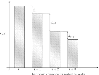
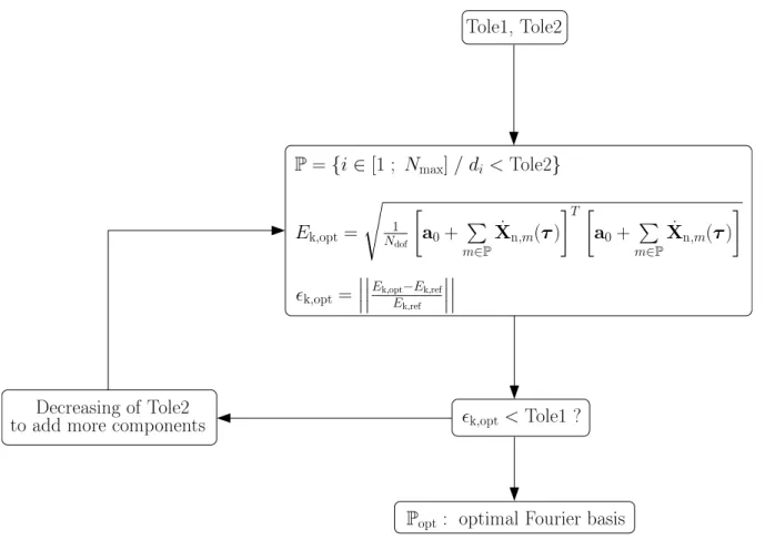
The analysis of the previous error ǫk,N allows the detection of the predominant harmonic com- ponents. The first step of this analysis is to introduce a target errorT ole1. Then, the harmonic components which “significantly” improve the mean square velocity are detected. As illustrated in Figure 3, all the gaps di = |ǫk,i+1−ǫk,i| are calculated and the highest correspond to the predominant components (i.e. by introducing a threshold T ole2). The optimized Fourier ba- sis is built by retaining only these predominant components. Then, the mean square velocity associated with the optimized Fourier basisEk,opt is calculated:
Ek,opt= X
m∈P
Ek,m (12)
whereP denotes the current optimal basis defined by:
P={i∈[1 ;Nmax]/di < T ole2} (13) Ek,opt is compared with the reference mean square velocity Ek,ref with the following relative error:
ǫk,opt=
Ek,opt−Ek,ref Ek,ref
(14) If the target Tole1 is not reached, the “less” predominant components associated with the “lower”
gaps di are added in the Fourier basis and P is updated. The final optimal Fourier basis Popt corresponds to the following set:
Popt ={i∈[1 ;Nmax]/di < T ole2, ǫk,opt< T ole1} (15) This method is illustrated in Figure 4.
3.3 Relevance of the optimized Fourier basis
In order to evaluate the relevance of the optimized Fourier basis, the surface acoustic power error is also analyzed. This analysis is conducted by performing the complete direct BEM calculation and is just presented to justify the use of the optimized basis. The main idea is to calculate the relative error between the optimized surface acoustic power and the reference calculated with all the harmonic components.
The surface acoustic power associated with the frequency ωi is of the following form:
WS(ωi) = 1 2ℜh
PS(ωi)X˙∗n,i i
(16)
000000 000000 000000 000000 000000 000000 000000 000000 000000 000000 000000 000000 000000 000000 000000 000000 000000 000000 000000 000000 000000 000000 000000 000000 000000 000000 000000 000000 000000 000000
111111 111111 111111 111111 111111 111111 111111 111111 111111 111111 111111 111111 111111 111111 111111 111111 111111 111111 111111 111111 111111 111111 111111 111111 111111 111111 111111 111111 111111 111111
000000 000000 000000 000000 000000 000000 000000 000000 000000 000000 000000 000000 000000 000000 000000 000000 000000 000000 000000 000000 000000 000000 000000 000000 000000 000000 000000
111111 111111 111111 111111 111111 111111 111111 111111 111111 111111 111111 111111 111111 111111 111111 111111 111111 111111 111111 111111 111111 111111 111111 111111 111111 111111 111111
00000 00000 00000 00000 00000 00000 00000 00000 00000 00000 00000 00000 00000 00000 00000 00000 00000 00000
11111 11111 11111 11111 11111 11111 11111 11111 11111 11111 11111 11111 11111 11111 11111 11111 11111 11111
000000 000000 000000 000000 000000 000000 000000 000000 000000 000000 000000 000000 000000 000000
111111 111111 111111 111111 111111 111111 111111 111111 111111 111111 111111 111111 111111 111111
harmonic components sorted by order
i i+ 1 i+ 2 i+ 3
di
di+1
di+2
ǫk,N
Figure 3: Detection of the predominant harmonic component
The surface acoustic power associated with the truncationN is given by:
WN =
N
X
i=1
WS(ωi) (17)
The reference acoustic power Wref is calculated with all the harmonic components:
Wref =WNmax (18)
Then, the acoustic power convergence is studied with respect to the number of retained harmonic component by introducing the following error:
ǫp,N =
WN −Wref Wref
with N = 1...Nmax (19)
The optimized surface acoustic power Wopt is calculated with the optimized Fourier basis:
Wopt =X
i∈P
WS(ωi) (20)
The relevance of this basis in the acoustic problem is evaluated with the error between Wopt
and Wref:
ǫp,opt=
Wopt−Wref Wref
(21) 3.4 Application to the single and multi-instability cases
In this section, the calculation of the optimal Fourier basis is conducted for the cases 1 and 2.
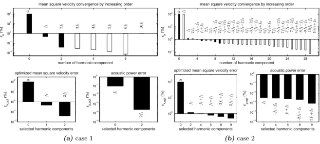
The dynamic response of the case 1 is composed of the fundamental frequencyf1 and several harmonic components 2f1, 3f1, 4f1, 5f1, 6f1and 10f1. By using the method detailed in Figure 4 (a), the mean square velocity convergence can be analyzed as shown in Figure 5. The higher gaps are detected for the zero order and for f1. By selecting these components, it is observed that the optimized mean square velocity error ǫk,opt (i.e. the relative error between the reference and the mean square velocity calculated with the optimized Fourier basis) reaches 0.48% as illustrated in Figure 5 (a). In order to try to quantify the relevance of the optimized Fourier basis
ǫk,opt =
Ek,opt−Ek,ref
Ek,ref
P={i∈[1 ; Nmax]/ di <Tole2}
Ek,opt = s
1 Ndof
a0+ P
m∈P
X˙n,m(τ) T
a0+ P
m∈P
X˙ n,m(τ)
ǫk,opt< Tole1?
P
opt: optimal Fourierbasis
toadd more omponents Dereasingof Tole2
Figure 4: Optimized Fourier basis calculation algorithm
over the acoustic response, the surface acoustic power error ǫp,opt is calculated with the same components. It is observed in the Figure 5 (a) that the acoustic power is well estimated with only few harmonic components with an error of 0.1%. Adding the less predominant harmonic component 2f1 provides a final errorǫk,optof 2×10⁻²% as indicated in Figure 5 (a). Moreover, the acoustic power error reaches 2×10⁻⁴%. So, the convergence of the optimized mean square velocity and acoustic power are in good agreement.
The focus is now on the optimal Fourier basis associated with the case 2 during the stationary regime. As previously explained, the Fourier basis of this case is more complex than for the single instability case. Figure 5 (b) shows the mean square velocity and the acoustic power errors for the optimal Fourier basis. For this case, the optimized mean square velocity convergence is slower due to the complexity of the spectrum. However, the iterative process allows to reach a tolerance of about 0.5% for ǫk,opt with only five harmonic components. The optimized Fourier basis is also suitable for the acoustic power with a final error of about 10−3%.
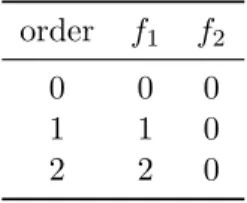
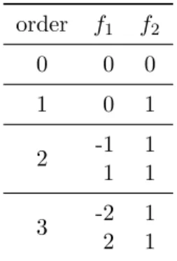
The optimal Fourier basis associated with the cases 1 and 2, calculated with a tolerance of 5×10⁻²% and 0.5% respectively, is listed in Tables 2 and 3.
4 Acoustic approximation method
The second level of approximation involves the radiations in free space which are calculated with the BEM for each frequency and each field plane. To avoid these calculations, an analytical expression of 3-D directivity of the radiating structure is first determined and several indicators
0 2 4 6 10−2
10−1 100 101 102
mean square velocity convergence by increasing order
number of harmonic component εk (%)
0
f1 2f1 3f1 4f1 5f1 6f1 10f1
0 1 2
10−2 10−1 100 101 102
optimized mean square velocity error
selected harmonic components
εk,opt (%) 0 f1 2f1
0 2
10−5 10−4 10−3 10−2 10−1 100
acoustic power error
selected harmonic components
εp,opt (%) f1 2f1
(a)case 1
0 4 8 12 16 20 24 28
10−1 100 101 102
mean square velocity convergence by increasing order
number of harmonic component εk (%)
0 f1 f2 2f1 -f+f12 f+f12 2f2 3f1 -2f+f12 2f+f12 -f+2f12 f+2f12 -3f+f12 3f+f12 -2f+2f12 4f1 -3f+2f12 -4f+f12 4f+f12 6f1 6f+f12 7f1 -5f+2f12 7f+f12 -7f+f12 -7f+2f12 8f+f12 -8f+f12 -9f+f12 -10f+f12 10f+f12
0 2 4 5 8 9
100 101 102
optimized mean square velocity error
selected harmonic components
εk,opt (%) 0 f2 -f1+f2 f1+f2 -2f1+f2 2f1+f2
2 4 5 8 9
10−5 10−4 10−3 10−2 10−1 100
acoustic power error
selected harmonic components
εp,opt (%) f2 -f1+f2 f1+f2 -2f1+f2 2f1+f2
(b)case 2
Figure 5: Iterative building of the optimized Fourier basis for the cases 1 and 2; black bar:
selected harmonic component; white bar: non selected harmonic component. (a): Case 1; (b):
case 2.
order f1 f2
0 0 0
1 1 0
2 2 0
Table 2: Optimal Fourier basis for the case 1 withT ole1=5×10⁻²%
are introduced to test its validity. Then, the acoustic power levels can be approximated with an appropriated propagation model for every field planes without the BEM.
4.1 Calculation of the directivity
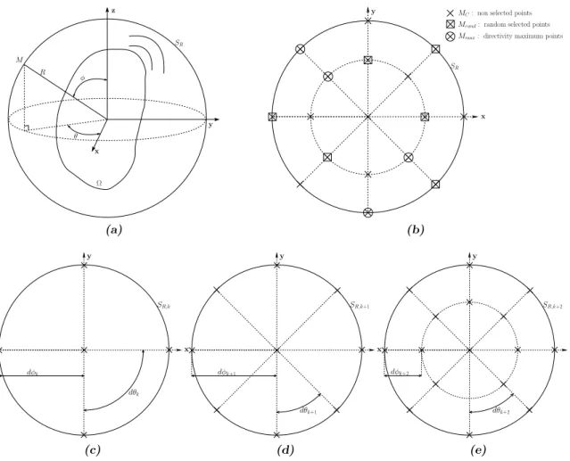
As previously explained, the first step of this approach is to well approximate the directivity. So, the focus is on the approximation of the directivity over a sphere which contains the radiating source. As seen in Figure 6 (a), the radiating source Ω is inside a sphere SR of radius R. The sound pressure overSRis denoted byP(θ, φ, ω), whereθ,φandR are the spherical coordinates of a point M over the sphere, and ω denotes the wave frequency. The acoustic intensity I is defined by:
I(θ, φ, ω) = P(θ, φ, ω)P∗(θ, φ, ω)
ρc (22)
whereρis the density of the air,cdenotes the speed of sound in dry air and the star corresponds to the conjugate. The acoustic intensity along a given direction Iaxe is also introduced:
Iaxe=I(θ0, φ0, ω) (23)
where (θ0, φ0) denotes a given direction which will be used as a reference and it corresponds to the direction along which the acoustic intensity I is maximum. Finally, the directivity h is
order f1 f2
0 0 0
1 0 1
2 -1 1
1 1
3 -2 1
2 1
Table 3: Optimal Fourier basis for the case 2 with T ole1=0.5%
calculated by:
h(θ, φ, ω) = I(θ, φ, ω)
Iaxe (24)
The function h provides the directions along which the source can radiate. In order to eval- uate this function, the Boundary Element Method is used. The sound pressure P(θi, φi, ω) is calculated for all the points (θi, φi)∈SRand the discrete directivityhbem(θi, φi, ω) is calculated.
4.2 Directivity polynomial fitting
The main point of this approach is to calculate an analytical expression of the directivity which can be evaluated for all points in free space. The previous BEM calculation only provides the directivity values for a finite number of points over the sphere SR. A simple way to approxi- mate this analytical function from its discrete values is to use a polynomial interpolation. The interpolation problem is to determine the optimal degree which provides the best analytical directivity function h:
h(θ, φ, ω) =
d
X
i=0 i
X
k=0
αikθkφi−k, with (θ, φ)∈R (25) whereαikdenotes the unknown coefficients of thed-order polynomial. In such a problem, the use of a high polynomial degree provides a well interpolated function over the calculation points but in some case, it generates high oscillations between these points: this is the well known Runge phenomenon. To avoid this phenomenon, the idea is to apply the polynomial interpolation over a part of the known values and then to evaluate the analytical function over all the points. This allows us to determine the best degree in which both minimize the interpolation error and avoid the Runge phenomenon.
The directivity interpolation is performed over 80% of all the points divided in a random set Mrand and a set composed of the directivity maximum points Mmax (Figure 6 (b)). Then, the interpolated functionh is evaluated over the whole set composed of the non selected points MC, Mrand and Mmax. The optimal polynomial degree is then determined by minimizing the error between the known values and the interpolated function. This problem takes the following form:
Find d∈Nminimizing
||h(M, ω)−hbem(M)||∞= max
(θi,φi)∈SR
d
X
i=0 i
X
k=0
αikθkiφi−ki −hbem(θi, φi, ω) withM = (θi, φi)∈SR
(26)
SR
y
x z
R M
θ
Ω φ
(a)
x y
SR
Mmax: directivity maximum points Mrand: random selected points MC: non selected points
(b)
x SR,k y
dθk dφk
(c)
x SR,k+1 y
dφk+1
dθk+1
(d)
x SR,k+2
dθk+2 dφk+2
y
(e)
Figure 6: (a): Draft of the radiating sourceΩin the sphereSR; (b): illustration of the selected points for the polynomial interpolation; (c)–(e): sphere refinement method; (c): SR,k,dθk,dφk; (d): SR,k+1,dθk+1,dφk+1; (e): SR,k+2,dθk+2,dφk+2.
However, it is important to note that the interpolation strongly depends on the directivity shape. In this paper, a preliminary work allows to use the polynomial fit. In the general case, preliminary BEM calculations have to be performed to identify the global features of the radiations. However, the previous method can still be applied by changing the interpolation type.
4.3 Directivity convergence criteria
The previous method explains how to evaluate the polynomial interpolation quality but does not provide information about the accuracy of the estimated directivity. By refining the sphere SR (i.e. by adding more BEM calculation points), it is possible to improve the interpolated directivityh. The issue is now to introduce a criterion to determine the optimal number of BEM calculation points to reach the best directivity. In this section, the focus is on the directivity convergence with respect to the number of BEM calculation points over SR.
4.3.1 Sphere refinement method
The first step consists of choosing an initial number of BEM calculation points. That is to say, to fix the refinement of the first sphere denoted by SR,1 which contains a “small” number of
points. For this first sphere, the directivity is calculated by using the interpolation processing method previously defined. Then, the sphere is refined by adding points over SR,1. The k-th sphere associated with the refinement k is denoted by SR,k and corresponds to the directivity hωk. As illustrated in Figures 6 (c),(d) and (e), the successive sphere refinements are of the following form:
• The sphere SR,k is built with the characteristic lengths: dθk;dφk
• The sphere SR,k+1 is built with the characteristic lengths: dθk+1 = dθ2k;dφk+1 =dφk
• The sphere SR,k+2 is built with the characteristic lengths: dθk+2 =dθk+1;dφk+2 = dφk+12 By successively decreasing the characteristic lengthsdθk anddφk, the number of points growth is not too fast and the optimal number of points is accurate. Moreover, it can be noticed that the spheres are imbricated. Thus, the BEM calculations only involved the added points between two refinement steps.
4.3.2 Global convergence
The directivity accuracy cannot be estimated over the current sphere because the interpolated directivity minimizes the least square error between the interpolated function and the known values over the sphere. That is why the directivity hωk is evaluated over an observation plane Pobs as illustrated in Figure 9. For the k−1-th sphere SR,k−1, the directivity hωk−1 is also evaluated over Pobs. The global convergence criterion aims at evaluating the error betweenhωk and hωk−1 overPobs denoted by ǫωh,k. The sphere refinement is stopped when the previous error reaches the initially fixed tolerance A1:
(ǫωh,k =||hωk(Mobs)−hωk−1(Mobs)||∞< A1
with Mobs = (θobs, φobs)∈Pobs (27)
4.3.3 Pattern convergence
The previous global criterion involves all the point of the observation plane Pobs. So, small localized gaps between two successive interpolated directivity are considered and thus this cri- terion is strict. A less restrictive way to estimate the directivity convergence is to analyze the directivity pattern over the field plane Pobs. The directivity hωk is evaluated over Pobs and the patternCω
k (which corresponds to the sphereSR,k) is detected:
Ckω(Mobs) =
(1 if hωk(Mobs)≥¯hωk(Mobs)
0 otherwise (28)
where the bar denotes the mean. For the reader comprehension, a draft of the pattern detection is given in Figure 9. The sphere refinement is stopped when the relative error between the patternsCω
k andCω
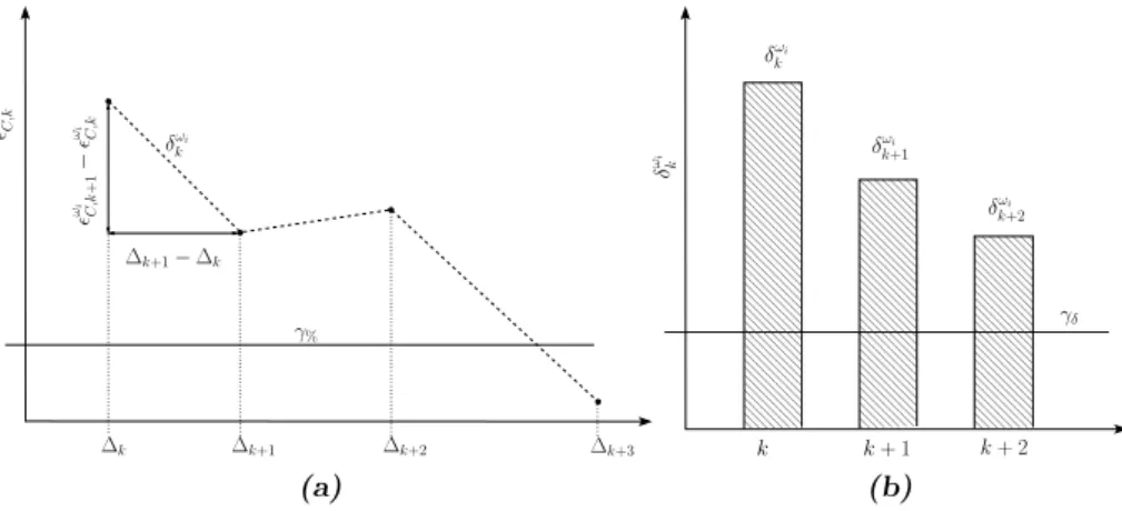
k−1, denoted byǫωC,k, reaches the tolerance γ% as illustrated in Figure 7 (a).
Moreover, the gradient of the relative errorǫωC,k must be less than the tolerance γδ to obtained the stabilization of the solution (see Figure 7 (b)). The relative error between two successive patterns takes the following form:
ǫωC,k= card{(θobs, φobs)∈Pobs/|Cω
k −Cω
k−1|= 1}
card(Pobs) (29)
where card denotes the number of elements of a given set. ǫωC,k corresponds to the percentage of added information between two successive refinements. It does not consider the values of the
ǫωi C,k
∆k+1 ∆k+2
∆k
δωki
ǫωi C,k+1−ǫωi C,k
∆k+1−∆k
γ%
∆k+3
(a)
00000 00000 00000 00000 00000 00000 00000 00000 00000 00000 00000 00000 00000 00000 00000 00000 00000 00000 00000 00000 00000 00000 00000
11111 11111 11111 11111 11111 11111 11111 11111 11111 11111 11111 11111 11111 11111 11111 11111 11111 11111 11111 11111 11111 11111 11111
00000 00000 00000 00000 00000 00000 00000 00000 00000 00000 00000 00000 00000 00000 00000 00000 00000
11111 11111 11111 11111 11111 11111 11111 11111 11111 11111 11111 11111 11111 11111 11111 11111 11111
00000000 00000000 00000000 00000000 00000000 00000000 0000
11111111 11111111 11111111 11111111 11111111 11111111 1111
k+ 1
k k+ 2
δωi k
δωki
δk+2ωi δωk+1i
γδ
(b)
Figure 7: Illustration of the directivity convergence criterion involving the detected pattern.
(a): Relative error between two patterns ǫωC,k with respect to the number of added points ∆k;
(b): draft of the error gradientδkω
directivity but only its shape over a given plane: that is why it is less restrictive than the first criterion. Therefore, the directivity convergence criterion has the following expression:
ǫωC,k≤γ% and δkω≤γδ withδωk = ǫωC,k+1−ǫωC,k
∆k+1−∆k (30)
where γ% and γδ denote the tolerance of the relative error and its gradient respectively, ∆k corresponds to the number of added points between the sphere SR,k+1 and SR,k:
∆k=card(SR,k+1)−card(SR,k) (31) These two criteria will be used to evaluate the directivity convergence for all the detected harmonic components ωi. The comparison between the two convergence results will allow to estimate the sensitivity of the approximated acoustic levels with respect to the convergence criterion. An overview of the directivity calculation is given in Figure 8.
4.4 Acoustic power level reconstruction
The Boundary Element Method provides the sound pressure at every point in the free space.
So, it is possible to directly calculate the level of acoustic pressureLωp,bem for a given harmonic component. In this simplified approach, the pressure is not known and the focus is on the acoustic power W and its levels LW = 10 log10(W/Wref), where Wref = 10−12 watt denotes the reference acoustic power. The aim of this method is to reconstruct the acoustic power and to calculate the levels LW to estimate the noise radiations in free space. The acoustic power of a given harmonic component ω associated with the directivity hωk is denoted by Wkω. The associated levels in decibels corresponds to the variableLωW,k. Three information are necessary to calculateWkω at every points:
• the directivity hωk which is calculated with the previously presented polynomial fit
• the input surface acoustic power vector Φω which corresponds to Φωi = 12ℜh
PS,iX˙n,i∗ i , where PS and ˙Xn denote the surface pressure and the surface normal velocity vectors respectively
A1 or(γ%, γδ)
BEMalulationoverSR,k:
alulation ofhωbem
alulation ofhωk
Polynomialt:
Diretivityonvergenetest:
ǫωh,k≤A1
δωk ≤γδ
or
ǫωC,k≤γ%
Optimaldiretivity:
hkω
Sphererenementproess:
SR,k←SR,k+1
False
Figure 8: Calculation of the interpolated directivity: polynomial fitting and convergence test
• a propagation model describing the noise level decrease with the distance from the source Involving the input surface acoustic power, it is directly obtained with the surface pressure calculated by the Boundary Element Method, and the surface normal velocity field calculated by temporal integration. The first approximation used in this approach is to consider that the radiating source Ω is a punctual source Ωp. That is to say, the source Ω generating the acoustic power vectorΦω is replaced with a punctual source Ωp with the scalar acoustic power Φωp. Ωp is located at the mean position of Ω and Φωp corresponds to the average ofΦω.
Moreover, a classical propagation model is to consider that the acoustic power in free spaceWkω decreases as R12
obs
where Robs is the distance from the source Ωp. Then, the acoustic power in free space is calculated with the following expression:
Wkω(M) = ΦωpSΩhωk(M)
R2obs (32)
whereSΩ denotes the surface of the source Ω. The variableM denotes a point in the free space and Robs is the distance of M from the punctual source Ωp. Then, the acoustic power levels LωW,k are calculated and compared with the sound pressure levels Lωp,bem calculated with the Boundary Element Method. The acoustic power is calculated for each harmonic components and the global acoustic power fieldWtot is obtained by superposition.