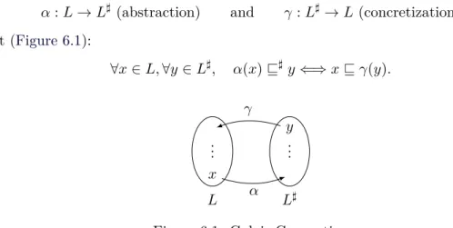
C'est pourquoi la seconde partie s'intéresse à l'analyse des relations linéaires (chapitres 5, 6, 7), cadre d'interprétation abstrait couramment utilisé, dédié à la génération automatique d'invariants sous forme d'inégalités linéaires sur les nombres de variables d'un programme. Il est accompagné d'un benchmark construit à partir de 102 cas tests issus de la littérature sur les problèmes d'invariant et de terminaison de boucle, et s'interface avec trois outils d'analyse de programme, utilisant différents algorithmes : Aspic, iscc et PIPS.
Linear Systems
Control-Command Critical Systems
Control-Command Systems
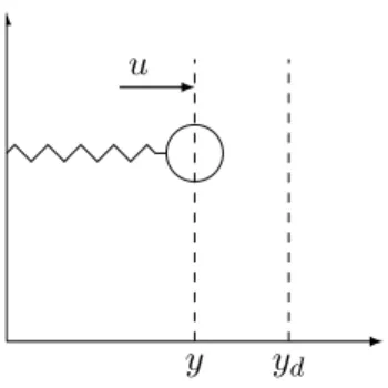
To design a control system, control engineers need to know exactly the effect that actuators have on the system. In the setting defined by internal statexp and input valuesup, outputyp (interpreted as a system action) follows Eq.
Open-Loop and Closed-Loop Controllers
Hardware implementation: either with a purely mechanical implementation - as is the centrifugal governor in Figure 1.1 - or with analog electronics. To implement a controller, it is necessary to discretize its internal state equation (1.1) to be able to recalculate its internal state xc at a fixed frequency:. 1.3) Typical frequencies for embedded systems are around 100 Hz.
Stability Proofs
Its name comes from the information path in the system: process input (e.g. fuel flow in jet engines) has an effect on process output (e.g. engine power), which is measured by sensors and processed by the controller; the result (the control signal) is fed back as input to the process, thereby closing the loop. Guaranteed performance even with model uncertainties, when the model structure does not perfectly match the real process and the model parameters are not accurate, unstable processes can still be stabilized.
Lyapunov Stability Proofs
Lyapunov Stability Theory
Various types of stability can be discussed for the solutions of differential equations that describe dynamical systems. Lyapunov functions are scalar functions that can be used to prove the stability of an equilibrium.
Motivating Example by Feron
The most important type is that which concerns the stability of solutions near the equilibrium point. Informally, a Lyapun function is a function that has positive values everywhere except at the equilibrium in question and decreases (or does not increase) along each trajectory of the differential equation f of the control system.
Open-Loop Stability Proof with Reals
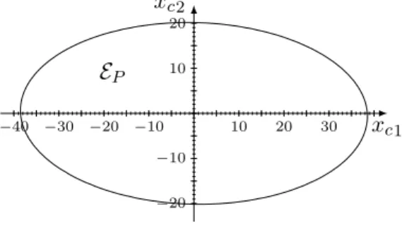
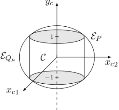
The correctness of this assertion stems from the fact that, given any value of µ ∈ [0,1], the domain EQµ is a solid ellipsoid, centered around 0, and whose intersection with the planes yc = 1 and yc =− 1 is equal to EP. This claim must be checked to ensure the correctness of the proof statements.
Proof Scheme with Limited-Precision Numbers
Formalism
- Functions Symbols
- Valuations
- Domains (Invariants)
- Expressions
- Instructions
- Invariant Propagation
Let F⊂R be the target set of limited-precision representations of real numbers (eg, floating-point numbers). This definition can be extended to evaluate the image of a domain d∈ DK, the result is also a domain of DK.
Translation Scheme
Unlike these arguments, propagators must be defined on the entire domain DK × IK, that is, for any precondition and instruction. Efforts should be made to make d¯′ have a similar form to d′ to match the proof argument p′ used in this instruction, if possible.
Translation Steps
- Converting Constants
- Converting Functions
In this case, p( ¯d,¯ı) would fall back to the universal domain, which is of course valid, but prevents us from providing any interesting proof further in the program. In other words, ifd˜′ is a postcondition for an instruction ˜ıon real numbers, on some conditional domain d¯, and d¯′ is a superset of d˜′ loose enough to support the arithmetic error verr, then ¯ ′ is a valid postcondition for ¯ı, the limited-precision counterpart of statement˜ı.
Translating Stability Proof Scheme to Floating-Point Numbers
- Automatic Translation
- Handling Constants
- Handling Functions
- End of Proof Scheme
- Closed-Loop Stability Proof Scheme with Floating-Point NumbersNumbers
- Alternative Limited-Precision Arithmetics
At the end of the proof scheme, the system is stable with floating-point numbers if and only if the inclusion. Unfortunately, these invariants are not enough to show that the stability condition holds at the end of the loop in the case of 64-bit floating-point numbers.
Linear Relation Analysis
Models, Programs, Verification
- Transition Systems
- Verification
- Properties
- Accessibility and Verification
- Model Checking
- Conservative Verification
- Program Models
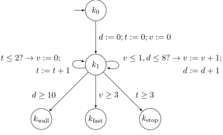
- Interpreted Automata
- Guard, Action, Guarded Command)
- Example
- Collecting Semantics
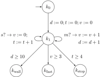
- Composition of Interpreted Automata and Observers
Each checkpoint is associated with a set of guarded commands that act on variables and lead to other checkpoints. An interpreted automaton is a triple α = (K,Com, kinit), where K is a finite set of control points, Com is a finite set of commands, and kinit ∈K is the initial control point. First, we define the parallel synchronous composition on interpreted automata: intuitively, two automata composed with parallel synchronization will execute commands together, provided the values of variables coincide on both sides - the idea is that a variable is either local to an automaton (and thus left unspecified in the other), or calculated in one automaton and read (and then left unspecified) in the other.
The synchronous product A × A′ of two interpreted automata A= (K,Com, kinit) and A′ = (K′,Com′, k′init) with a common set of variables X is the automaton (K×K′ ,Com×,( kinit, k′init)) where. The observer P is an interpreted automaton O that works on a partitioned set of variables X⊎X′ and such that.

Abstract Interpretation
- Introduction
- Principles of Abstract Interpretation
- Abstract Domains
- Abstract Operations
- Widening and Decreasing Sequence
- Abstract Interpretations of Interpreted Automata
- Approximating Numeric Sets
- The Sign Lattice
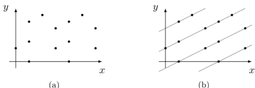
- The Lattice of Linear Congruences
- The Lattice of Intervals
- The Lattice of Convex Polyhedra
- Particular Polyhedra
- Semi-Linear Sets and Presburger Arithmetic
- Uses of Numerical Variables Analysis
- Verifying Inaccessibility
- Invariant Synthesis
The initial fixed-point equation on concrete values is then associated with an abstract fixed-point equation, which must be solved in the abstract domain. This theorem implies that to compute an over-approximation of the smallest fixed point of a concrete function F, we can choose or build an abstract function G satisfying equation (6.2), the smallest fixed point of G in the abstract be able to calculate a grid and concretize the result . An interpretation of guards in the abstract grid, that is, an effective way of associating an abstract valueg♯ to each guardg, such that.
A rough abstraction consists in associating each variable with an abstract value in the grid represented in figure 6.2. In some applications, it is necessary to add auxiliary counters to the program and in the analysis of their behavior.
The Lattice of Polyhedra
- Two Representations
- Linear Constraints
- Non-Canonicity of Constraint Systems
- Generators
- Non-Canonicity of Generator Systems
- Link between the Two Representations Satisfaction of Constraints by the Generator ElementsSatisfaction of Constraints by the Generator Elements
- Minimization of Representations
- Computing the Dual Representation
- Principle of Motzkin’s Algorithm
- Optimizations
- Operations on Polyhedra
- Tests
- Intersection
- Convex Hull
- Applying Actions, Projections and Affine Transformations
- Widening
- Limited Widening
- Analysis Example
- Existing Libraries
- PolyLib
- NewPolka
- PIPS/Linear
In this paragraph, we focus on the non-canonicality of the representation with linear constraints. The previous proposal allows for simplification of representations and identification of mutually redundant constraints at the expense of computational saturations (i.e. the product of the constraint matrix with the generator matrix). To avoid this problem, the extension operator [Hal79] uses the notion of mutually redundant constraints (see Definition 7.5): a system of constraints P∇Q is formed by constraints Q that are mutually redundant in P with a constraint in p.
Each control point of the automaton is associated with a polyhedron (see Figure 7.9), as shown in Section 6.3. The Integer Set Library†11 (orisl) [Ver10] is a thread-safe C library for manipulating sets and point relations of integers bounded by ane constraints:. 7.1) Descriptions of sets and relations can include both parameters (s in equation (7.1)) and existing quantitative variables (z in equation (7.1)).
ALICe: A Framework to Improve Affine Loop Invariant Computation
Invariant Computation
Most of the usual analysis techniques consist of starting from a set of assumed predicates about a particular control position in the transition system, and then spreading them to other positions by evaluating the effect of each transition on the predicates. We propose a toolkit that compares these tools on a common set of small-scale, previously published test cases and to test the sensitivity of these tools to different encoding schemes.
The ALICe Framework
- Program Model
- Test Cases
- Supported Tools
- Heterogeneity of Tools
- Translation Tools
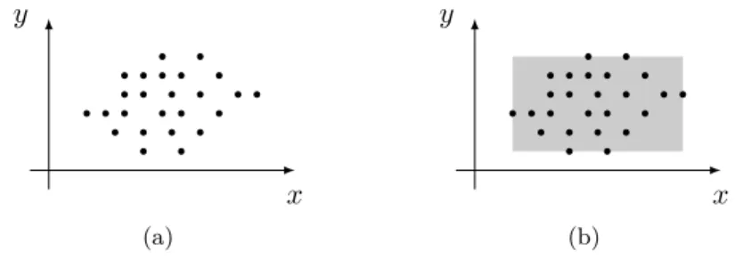
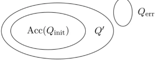
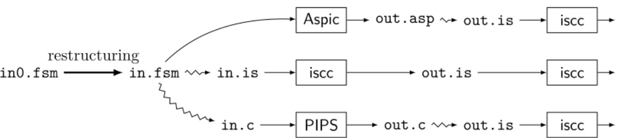
The tool successfully analyzes the model if and only if the calculated invariant, an overestimation of the attainable states, does not intersect with the set of error states Qerr. However, as all analytical tools used within ALIC are primarily for forward analysis (see Section 8.2.5), this is not explored further. Use iscc to check if the intersection of the model error region and the invariant computed by the analyzer is empty, ie.
This regular expression represents the structure of generated C code: unions are translated into conditional branches (if (and asterisks into loop statements (while (rand()). Dummy string instructions are also injected, to keep track of names of variables and control points of the original model in the produced C code.
Results for the Raw Test Cases
Conversely, it is possible to use ALICe to analyze simple models written in C by first translating them into fsm automata using C2fsmutility. It is therefore important to generate a simple regular expression to avoid producing unnecessarily complicated C code. Anisccrelation is produced directly from the fsm model without the need for restructuring, renaming or control state tracking.
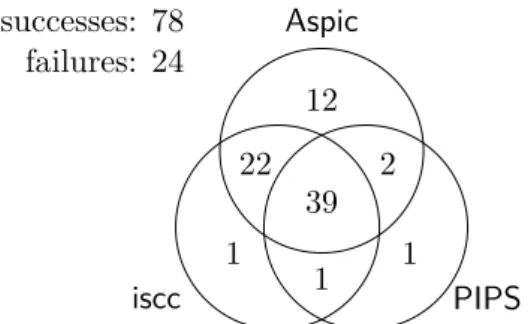
This ranking is not a total ranking because no tool is strictly better than another: for each tool, there is at least one pattern that is successfully analyzed by this tool alone, as shown in Figure 8.5;. Finally, despite his successes, Aspichas has more difficulty dealing with transitions with complex formulas, which he is unable to speed up.
Model-to-Model Restructuring Transformations: Sensitivity to
- Control-Point Splitting Heuristic
- Algorithm
- Correctness Theorems
- Partition Choice
- Guard-Based Control Partitioning
- Reduction to a Unique Control Point
- Combining Restructuring Transformations
- Impact of Restructuring Transformations on Experimental ResultsResults
These inaccuracies accumulate if there are structures in the automaton with two or more loops involved in the same control point. The checkpoint partitioning algorithm presented here is a refactoring that aims to achieve these two goals. We consider a general automaton m= (X, K,Trans, Qinit, Qerr) and its imageM/k obtained by splitting control nodes∈K ofm through the control point splitting algorithm.
In the general case, partitioning a control into components adds not only m control states to the automaton, but also up to m2 transitions between the newly created controls — from any control to any control —; the larger size and more complex structure will increase the analysis complexity. Indeed, some relations on control points may or may not be expressed in terms of any constraints, depending on the control point encoding.
Computing Invariants with
Transformers: Experimental Scalability and Accuracy
- Generation of Invariants with Transformers
- Generation of Transformers by PIPS
- Generation of Invariants
- Modularity and Accuracy: Experimental Results
- Tools Used
- Impact of Cycle Nesting on Convergence
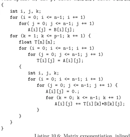
- Interprocedural Analysis or Inlining
- New Improvements in Transformer Computation
- Concurrent Loops
- Arbitrary-Precision Numbers
- Other Improvements in Transformer Computation
- Iterative Analysis
- Periodicity
- While-If to While-While Conversion
- Experimental Evaluation of the Improvements
- Impact of Improvements for PIPS
- Analysis of PIPS Failures
With equation (10.1), they are performed later in the precondition space and each elementary pass is used as the last pass. Note that the precondition of the nth loop Pn∗, which can be calculated more precisely by equation (10.1), affects the (n+ 1)th transformer Tn+1 in two different ways. Note that periodic analysis (Section 10.4.2), which is not shown in Table 10.3, does not improve any test case currently in ALICE.
Sizes in number of lines are shown in Table 10.4 for FAST files and forCE files generated by fsm2c. Note also that the PIPS execution times in Table 10.3 differ greatly from those shown in 112 .
Conclusion
Utilisés séparément ou ensemble, ils permettent d'améliorer significativement les résultats d'analyse et aident à identifier les forces et les faiblesses de chaque outil d'analyse. La portée d'ALICE peut également être étendue, d'une part en ajoutant de nouveaux modèles à la base de données des cas de test, et d'autre part en supportant davantage d'outils d'analyse. Il convient également de vérifier que les outils d'analyse génèrent des invariants réalistes, par exemple en liant un invariant minimum pour chaque cas de test.
Un outil d'analyse ne sera considéré comme correct que si les invariants qu'il génère sont des sur-ensembles des invariants minimaux. Enfin, même si les améliorations apportées au calcul des invariants par transformateurs ont permis d'améliorer significativement les résultats en PIPS, le coût de calcul le rend peu pratique pour l'analyse de gros programmes.
Bibliography
Verification of Real-Time Systems using Linear Relation Analysis.Formal Methods in System Design August 1997. In Tales and Compilers for Parallel Computing, volume 2017 of Lecture Notes in Computer Science, pages 97–111.