Amélioration des performances des radars à ondes de surface HF par l'étude d'une antenne compacte et l'application d'un filtrage adaptatif. De nombreuses idées sur l'antenne HF compacte elle-même devraient être testées à l'avenir.
Cr´ eation d’une base de donn´ ees d’´ echos de mer simul´ es
La deuxième partie de cette thèse vise donc à réduire l'influence du fouillis de mer pour améliorer les capacités de détection des radars à ondes de surface HF. Pour réduire l'influence du fouillis de mer, il est tout d'abord indispensable d'avoir une bonne connaissance des caractéristiques du fouillis de mer.
D´ eveloppement et validation d’un algorithme de filtrage r´ eduisant le fouillis de mer
Introduction to HFWSR
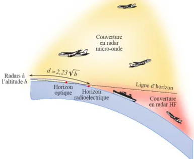
In general, they are microwave radars, that is, frequencies on the order of a few gigahertz and wavelengths of about the centimeter. Nevertheless, they are limited by the physical propagation properties of the very high-frequency waves.
RADAR HISTORY 3
Radar History
In the mid-1930s, advances in electronics brought concrete applications. On the one hand, the principles of physical radar have not changed significantly since the end of World War II.
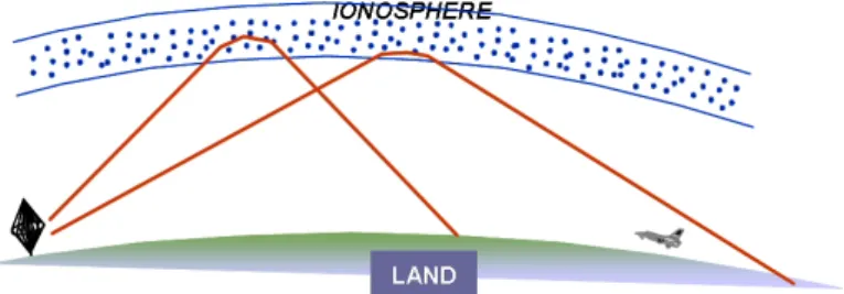
Over-the-horizon radars
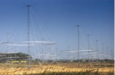
This is an example of an HF airwave radar called Nostradamus, developed by French researchers in ONERA. It is an experimental system based on an original concept of monostatic radar consisting of 3 branches.
OVER-THE-HORIZON RADARS 7 2 Surface wave radars
The country also has a bistatic HF surface wave radar called SECAR, in the north of the country, to monitor the Torres Strait. Additionally, much work is being done on the feasibility of a bistatic or multistatic HFSWR configuration.
General description of the HF surface wave radar system
Australia has achieved a position of world leadership in OTH Radar through the development of the Jindalee OTH airborne radar system at Alice Springs in central Australia, by the Australian Defense Science and Technology Organization (DSTO). This could have serious consequences for the safety and security of French people, for the environment and for the interests of the country in general.
GENERAL DESCRIPTION OF THE HF SURFACE WAVE RADAR SYSTEM 9
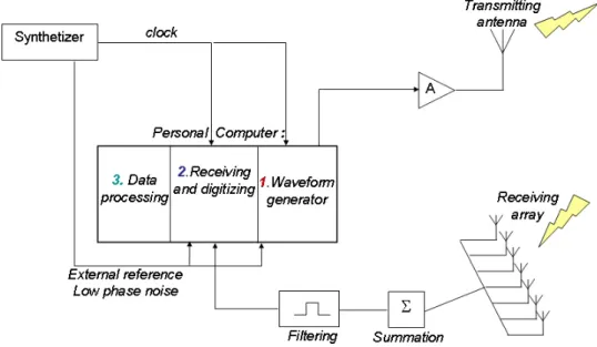
On this example of receiving part of the coastal HF radar, there are coherent receivers at the output of each antenna. The application of digital signal processing is practical because of the rapid progress in both digital hardware and software development.
Radar Equation
The signals are then digitally down-converted to complex baseband where all the necessary filtering, beamforming, Doppler analysis, detection, tracking, noise suppression and other signal processing operations are performed.
RADAR EQUATION 11 R : Range of the target in m
Radar functioning principle
RADAR FUNCTIONING PRINCIPLE 13 frequency, called ”carrier frequency” through an amplifier and a transmitting antenna
Radar processing
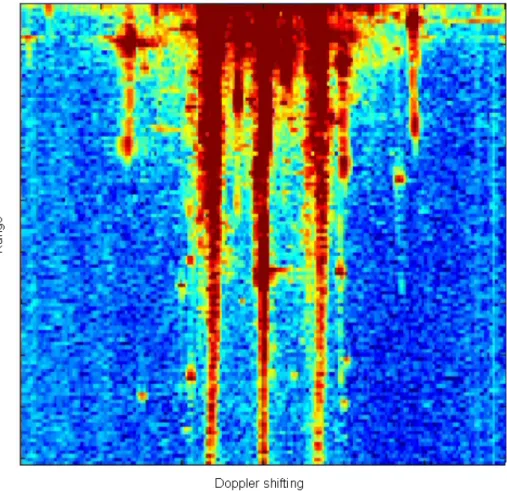
RADAR PROCESSING 15 Doppler shifting can be obtained. In reality, the processing step is a bit more complicated
Note that the received signal is reduced compared to the transmitted signal, this attenuation is represented by the factor A. RADAR PROCESSING 17 Next, it is now possible to find the received signal at time t for each iteration i.
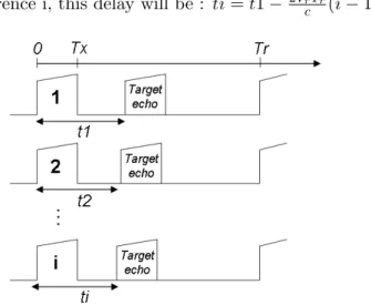
RADAR PROCESSING 17 Then, it is now possible to find the signal received at the instant t for each recurrence i
These successive samples are spaced out at least with a repetition, the Fourier transform then consists of applying a discrete Fourier transform where the sampling period is Tr. The Fourier transform is able to put the received samples back in phase, and this for each Doppler shift.
RADAR PROCESSING 19
In fact, we note, in equation number 1.3, that the term A4 corresponds to the replica of the transmitted code that is temporally shifted with the delay of the target ego (we previously assumed that the received code is not distorted by the target velocity). As shown in figure 1.16, side lobes are 26 dB above the highest correlation peak, which is well the double of a simple cardinal sine (cf. figure 1.13).
RESULTS AVAILABLE AFTER RADAR PROCESSING 23 Range resolution The range resolution corresponds to the minimum distance between
Results available after radar processing
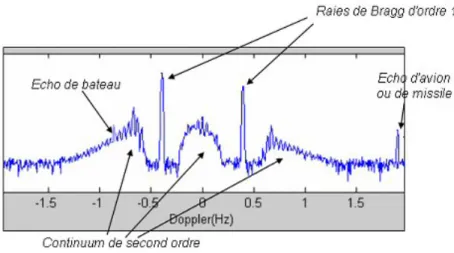
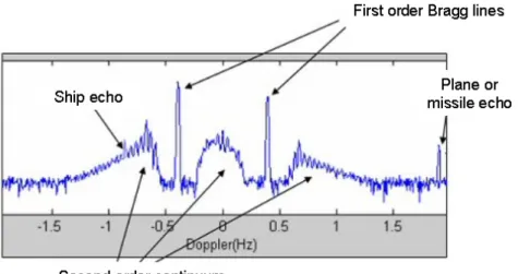
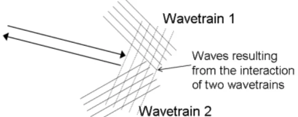
Echoes coming from sea disturbances appear as two lines called Bragg lines1 (the interaction between HF waves and sea waves will be described in more detail in Chapter 4). Spectral analysis of the return signal coming from marine reflections suggested a Doppler spectrum characterized by two dominant peaks surrounded by a continuum.
MAJOR CONSTRAINTS OF THE HF SURFACE WAVE RADAR 25
Major constraints of the HF surface wave radar
In the case of shipboard radars, electromagnetic problems can occur between the radar system and the ship's HF equipment. It is also important to consider the matching problems associated with coupling effects between the metallic environment of the ship and the antennas.
CONCLUSION ABOUT HF SURFACE WAVE RADARS 27 1.9.5 Disturbing ionospheric clutter
Conclusion about HF surface wave radars
First, a list of required characteristics to be respected will be described in detail and several examples of common HF antennas will be presented in order to understand the issue well. Then a base antenna is conceived and modeled to assess whether the initial performance meets the required specifications.
Definition of specifications needed for HFSWR antennas
DEFINITION OF SPECIFICATIONS NEEDED FOR HFSWR ANTENNAS 31 advantage but we know that for small antennas, the radiating power being low and due to
When a surface wave is horizontally polarized, the electric field of the wave is parallel to the sea surface and, therefore, is constantly in contact with it. On the other hand, when the surface wave is vertically polarized, the electric field is vertical to the sea surface and simply dips in and out of the surface.
COMPACTING USUAL HF ANTENNAS SIZE 33
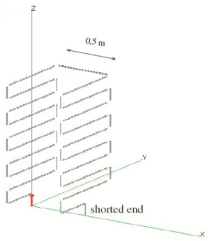
Compacting usual HF antennas size
The following Figure 2.3 presents commercial antennas used in the SeaSonde system developed by CODAR Ocean Sensors. On the left part of the image, the receiving antenna is composed of three elements attached to a passive vertical monopole mounted on a support pole.
COMPACTING USUAL HF ANTENNAS SIZE 35 The total size of this superdirective antenna is not specified on the advertising brochure
COMPACTING REGULAR HF ANTENNAS SIZE 35 The total size of this superdirective antenna is not specified on the advertising brochure. Sky-Cross antennas are based on the MLA technology that enables engineers to design high performance, multi-mode, multi-frequency antennas that can be hidden in a mobile enclosure.
COMPACTING USUAL HF ANTENNAS SIZE 37 Narrowband and broadband MLA MLA antennas are configured into two distinct
With reference to the desired antenna size, this compact antenna can be considered an electrically small antenna. The first work on the fundamental limits of electrically small antennas was done by Wheeler in 1947 [6].
COMPACTING USUAL HF ANTENNAS SIZE 39
In 1996, Mac Lean [9] proposed a simple formulation for the minimum quality factor achievable with an electrically small antenna. The MLA can be considered as an RLC type circuit and then its bandwidth related to the quality factor and its VSWR can be calculated using the following formula.
COMPACTING USUAL HF ANTENNAS SIZE 41 3.5 Efficiency of small radiating elements
Based on the similarity principle transferred to HF frequencies, we define a basic antenna that will be optimized and call it "generic antenna".

COMPACTING USUAL HF ANTENNAS SIZE 43
He studied the case of a microstrip meander line antenna used for mobile design equipment at 1.5 GHz. The current spots are in phase with the four vertical sections that radiate high current into the winding line.
Modeling of the generic antenna
To simulate the functioning of the antenna and to calculate all interesting values for its characterization, we use the integral representation of the electric field, associated with the Method of Moments. MODELING OF THE GENERIC ANTENNA 47For a wire structure we can present the Pocklington integral equation, which gives the.
MODELING OF THE GENERIC ANTENNA 47 For a wire structure, we can present the Pocklington integral equation, which is the
One of the main tasks in a particular problem is the choice of fn and wn. MODELING THE GENERIC ANTENNA 49 Actually, meshing is not a simple step because there is a precise number of segments.
MODELING OF THE GENERIC ANTENNA 49 In fact, meshing is not a simple step because there is a precise number of segments
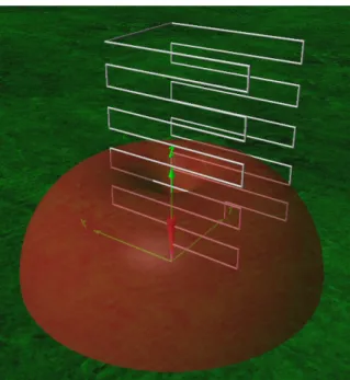
The theoretical maximum profit of the MLA can be calculated thanks to the Harrington formula (see 2.1). The dimensions of the generic antenna can be enclosed in a sphere that has a radius of approximately 1.059 m as shown in figure 2.12.
MODELING OF THE GENERIC ANTENNA 51
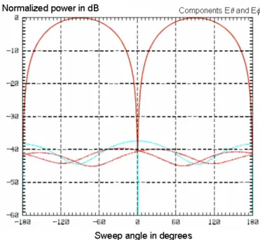
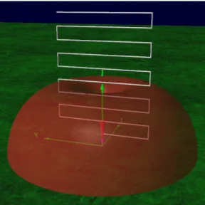
A handy tool available with NEC-2 version 4 is the 3D viewer which represents the results of the radiation model in 3 dimensions (see figure 2.14). The generic antenna has a radiation pattern that closely resembles that of a monopole antenna, for each frequency.
MODELING OF THE GENERIC ANTENNA 53 3.2 Simulations results by France Telecom
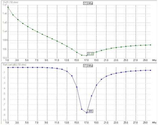
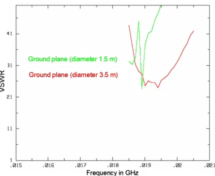
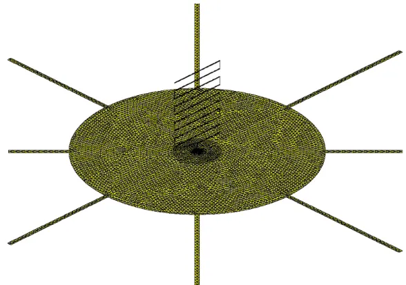
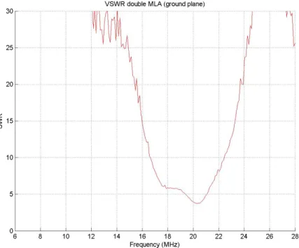
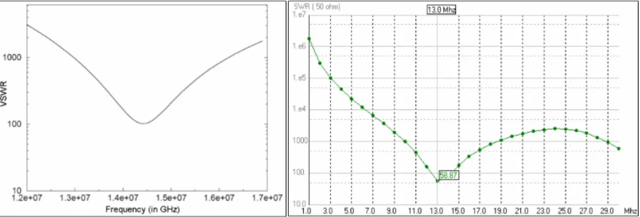
The instabilities are due to the small size of the ground plane, which is < λ/10. As for radiation pattern simulations, this has been done for 19.5 MHz with the ground plane having a diameter of 3.5 m.
MODELING OF THE GENERIC ANTENNA 55
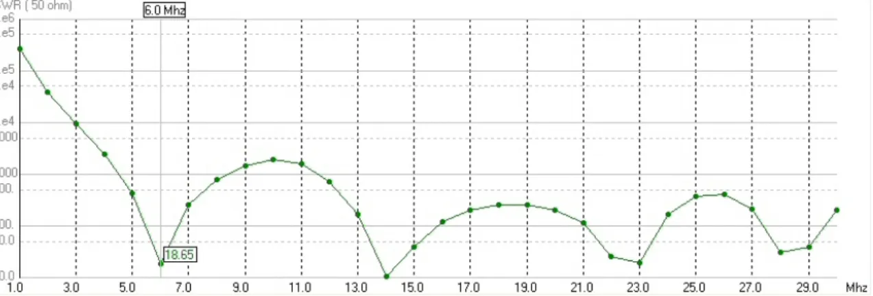
At this frequency, with an extended 2.8 m diameter ground plane, the VSWR is about 1.97, which is a good value. MODELING OF THE GENERIC ANTENNA 57For the radiation pattern, shown for the extended 2.8 m diameter ground plane of.
MODELING OF THE GENERIC ANTENNA 57 For the radiation pattern, displayed for the extended 2.8 m diameter ground plane on
The next step of the study will involve optimization of the generic antenna design to obtain the best possible performance in the smallest possible dimensions. Despite minor differences between the modeling results of the two codes previously used for the generic antenna, we have the general trend.
Search for parameters influencing antenna performance
SEARCH FOR PARAMETERS INFLUENCING ANTENNA PERFORMANCE 61
If we increase the distance between the first turn and the ground (a=0.2 m and 0.3 m), results are not improved. When the step is reduced (e1=0.05 m and 0.025 m), the results are mediocre and by testing irregular step, which means a variable distance between branches, we do not have a good surprise.
OPTIMIZATION OF THE INFLUENCING PARAMETERS 63
Optimization of the influencing parameters in order to combine compactness and performance
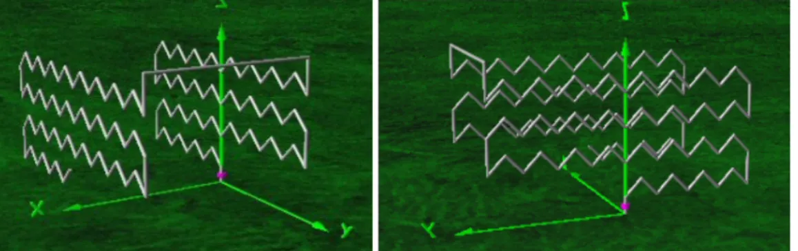
Because of the radiation resistance that can be increased, the reactances can be made to equalize each other in balanced and unbalanced current conditions. We tested the distance between the two parts of the antenna (10, 20 and 50 cm), tried to start the second structure and finally added a metallic wire between both.
OPTIMIZATION OF THE INFLUENCING PARAMETERS 65
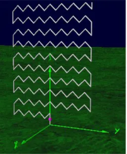
Doubling the structure had a favorable effect on the VSWR value, but not on the resonant frequency. OPTIMIZATION OF INFLUENTIAL PARAMETERS 67 A double MLA prototype was then produced by a French company specializing in antennas.
OPTIMIZATION OF THE INFLUENCING PARAMETERS 67 The double MLA prototype has then been built by a French firm, specialized in antennas,
The only way to significantly shift the resonant frequency is to significantly increase the overall length of the antenna. OPTIMIZATION OF THE INFLUENTIAL PARAMETERS 69 parts of the antenna by means of kind of zigzags.
OPTIMIZATION OF THE INFLUENCING PARAMETERS 69 parts of the antenna by means of kind of zigzags. In fact, horizontal wires do not contribute
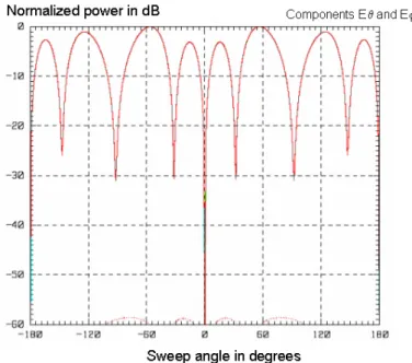
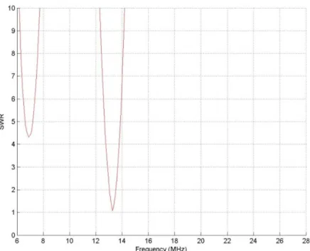
In fact, the resonant frequency is well shifted to the lower frequencies as shown in Figure 3.10, which means a frequency of 14 MHz, but the corresponding VSWR value is about 32. If we simulate the radiation pattern of the sinusoidal antenna at 14 MHZ, we have typical patterns with a maximum gain of 4.61 dBi in a seaward direction.
OPTIMIZATION OF THE INFLUENCING PARAMETERS 71
Compared to the twin prototype, we can assume that the length of the twin structure has been bent to obtain the sinusoidal antenna (see Figure 3.14). New experiments have been done with this prototype, with an extended ground plane of 8 long copper cables, and there is a natural impedance corresponding to approximately 13 MHz, as shown in Figure 3-15.
OPTIMIZATION OF THE INFLUENCING PARAMETERS 73
Besides the fact that the segment length of the sinusoidal antenna is very small, an additional problem concerns the low frequencies used in this study. The line length and connection point both need to be calculated from the load impedance.
OPTIMIZATION OF THE INFLUENCING PARAMETERS 75 to be nearly lossless; it may be open circuit, or short circuit, or indeed terminated in a
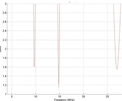
In order to verify the efficiency of individual matching, we performed experiments with a sinusoidal antenna. In this Figure 3.20 we see a real improvement in the VSWR value of the sine antenna at different frequencies.
SIMULATION AND REALIZATION OF FINAL ANTENNA PROTOTYPE 79 This sinusoidal antenna has quite good characteristics so far, mainly when used with
Simulation and realization of final antenna prototype fit- ting specifications
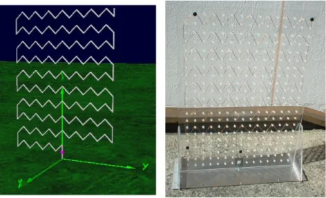
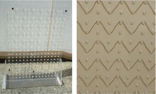
The resonant frequency around 6 MHz is the most interesting because of the ability to respond to specifications. In the following image 3.23 we can see the height difference between the biconical antenna of the HF skywave radar Nostradamus (height: 8 m) and the new prototype (height: 1.35 m).
SIMULATION AND REALIZATION OF FINAL ANTENNA PROTOTYPE 81 on figure 3.24 show that 5 resonant frequencies can be found : 5 MHz, 12.5 MHz, 18 MHz,
The exact design of the prototype can be found in Appendix 5.6.4 at the end of the document. The earthing of the box is made of aluminum and has practical handles for carrying the box.
SIMULATION AND REALIZATION OF FINAL ANTENNA PROTOTYPE 83 The connector is either a type 7/16, either a type N to connect easily the antenna to
SIMULATION AND REALIZATION OF FINAL ANTENNA PROTOTYPES 83 The connector is either 7/16 type, or N type to easily connect the antenna. SIMULATION AND REALIZATION OF THE FINAL ANTENNA PROTOTYPE 853.3.2 Validation of the prototype in a classical radar configuration.
SIMULATION AND REALIZATION OF FINAL ANTENNA PROTOTYPE 85 2 Validation of the prototype in a classical radar configuration
Potential targets such as aircraft are illuminated by the HF wave transmitted by the biconical transmitting antenna and they scatter a portion of this incident wave to the receiving radar system. In the experiment, the target signals are received by another large biconical antenna, an active monopole antenna (1 m high) and by the compact HF antenna prototype.
SIMULATION AND REALIZATION OF FINAL ANTENNA PROTOTYPE 87
Differences between SNR are not the same between antennas for each target as shown in the resulting figures. The target on the right is more visible with the biconical antenna and less so with compact prototype or monopole antenna.
SIMULATION AND REALIZATION OF FINAL ANTENNA PROTOTYPE 89 image corresponding to the compact HF antenna and less visible or totally absent on other
SIMULATION AND REALIZATION OF THE FINAL ANTENNA PROTOTYPE 89image that corresponds to a compact HF antenna and is less visible or completely absent on another. SIMULATION AND REALIZATION OF THE FINAL ANTENNA PROTOTYPE 91 We performed tests with a compact prototype in a receiving configuration close to the sea, but.
SIMULATION AND REALIZATION OF FINAL ANTENNA PROTOTYPE 91 We made tests with the compact prototype in receiving configuration near sea but the
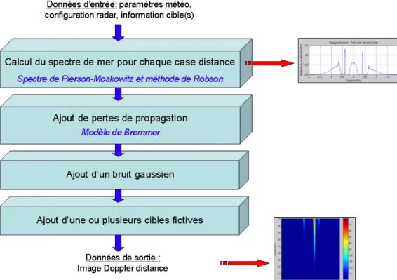
The purpose of this part is to obtain simulated sea echoes for any event (frequency, wind force, current velocity, etc.). The first step is to study properties of ocean echoes and better understand interactions between HF waves and sea surface and then implement an algorithm for the automatic generation of simulated data.
Characteristics of sea echoes
CHARACTERISTICS OF SEA ECHOES 95
This second-order continuum can confuse the spectrum and make detection impossible. If appropriate signal processing can reduce the effect of this second-order Bragg clutter, radars will be able to detect smaller boats or low-flying aircraft.
CHARACTERISTICS OF SEA ECHOES 97
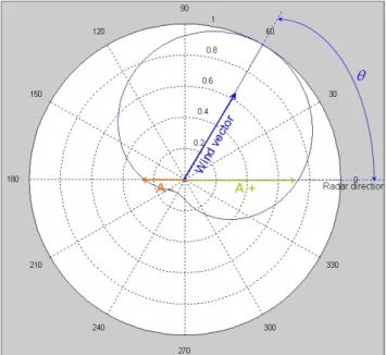
This wind direction can be obtained thanks to the ratio between the first order Bragg lines in the sea spectrum. The following formula 4.1, worked out by Maresca, relates the ratio between the energies contained in the dominant second-order and first-order Bragg lines to the mean square height of sea waves.
CHARACTERISTICS OF SEA ECHOES 99
Assuming that sea waves are generated by wind at sea level, the root mean square height of the waves can be related to the wind speed. Thanks to this empirical relationship, wind maps can be constructed, usually wind directions are represented by arrows on a geographical map, the size of the arrow being proportional to the wind speed.
SEA SPECTRA MODELING 101
Sea spectra modeling
This cardioid pattern gives the relative values of the receding (A-) and approaching (A+) components of the waves, as shown in Figure 4.9. From this pattern, the relative amplitude of the Bragg lines is known, as shown in Figure 4.10.
SEA SPECTRA MODELING 103 the way of propagation on this direction can not. The way of getting round this problem
To calculate second order cross section, two infinities of wave vectors k~1 and k~2 are used such as k~1+k~2=−2k~0. It is then possible to plot reflectivity of first and second order Bragg clutter as a function of the Doppler frequency.
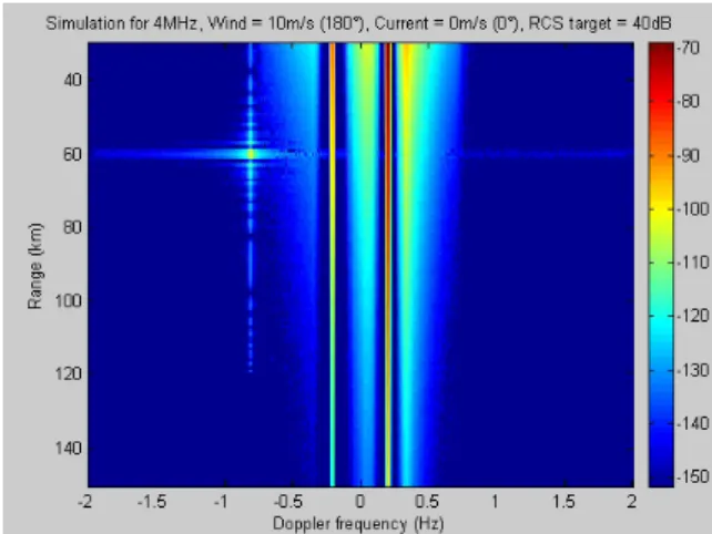
SEA SPECTRA MODELING 105 a low frequency of 4 MHz and a wind velocity of 4 m/s. Other considered parameters are
Creation of a simulated sea echoes database
CREATING A DATABASE OF SIMULATED MARINE ECHOES 107 means that we have the Doppler dimension but no information about it.
CREATION OF A SIMULATED SEA ECHOES DATABASE 107 means that we have the Doppler dimension but we do not have information about the
Most frequent range of results displayed: This is the last most frequent range displayed on the Doppler range image. Current direction (in degrees): This is the angle between the radar direction and the current direction.
CREATION OF A SIMULATED SEA ECHOES DATABASE 111 2.3 Target parameters
In fact, as the range increases, the sea echo level decreases due to the R4 term in the denominator of the Radar Equation. CREATING A DATABASE OF SIMULATED SEA ECHOES 113 For each frequency, we can calculate the loss versus distance curve.
CREATION OF A SIMULATED SEA ECHOES DATABASE 113 For each frequency, we can calculate the losses curve in function of the distance. The
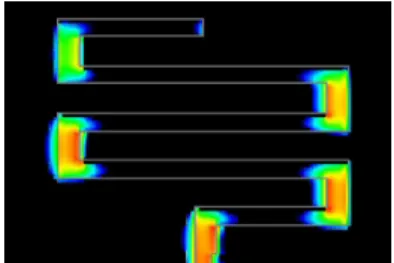
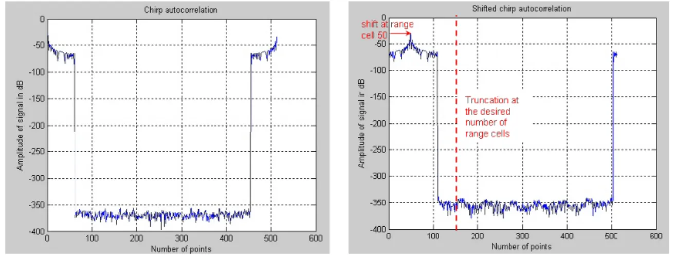
A Gaussian noise is added to the entire image, it is a random noise, the level of which is calculated thanks to the noisy part of the Radar Equation, i.e. See an example in Figure 4.20, where a chirp autocorrelation is generated at 512 points and moved to range cell 50 to obtain a location of the corresponding fic range.
CREATION OF A SIMULATED SEA ECHOES DATABASE 115 velocity and the frequential resolution, it is simple to determine the Doppler cell number
The problem is that these modeled data are really different from measured data because they are not propagated through the radar equipment and they are not processed by the Doppler range processing step. Thus, simulated spectra are "clean" because they are not affected by the equipment default and by the processing effect, which means that they do not have correlation or Doppler side lobes.
CREATION OF A SIMULATED SEA ECHOES DATABASE 117
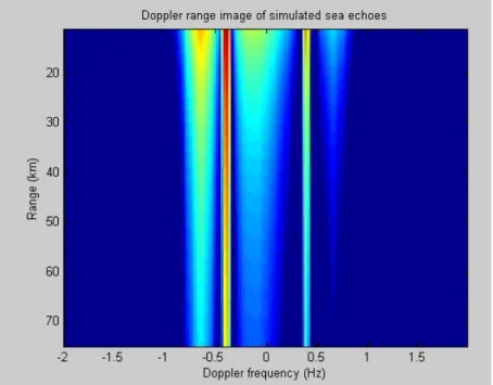
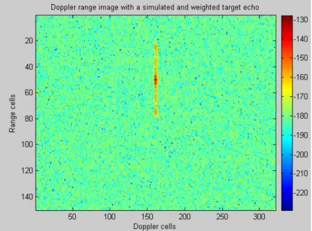
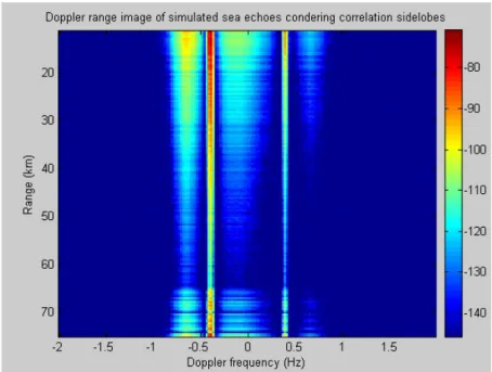
For the modeled data to be affected by Doppler processing, it is also possible to consider Doppler sidelobes in the same way as we did for the target simulation (see 4.3.6). On the following figure 4.24, this is a final Doppler range image of simulated ocean echoes where distance and Doppler processing effects are taken into account.
ANALYSIS OF THE SIMULATED SEA ECHOES DATABASE 119
Analysis of the simulated sea echoes database
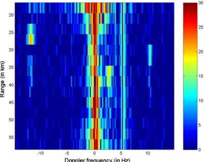
In Figure 4.27, at 10 MHz, the sea disturbance is very disturbing, as it is spread over the entire Doppler cells between -1 Hz and + 1 Hz. A target could not be detected in this Doppler interval unless its level was higher than the level of the Bragg lines due to strong RCS.
ANALYSIS OF THE SIMULATED SEA ECHOES DATABASE 121
It is interesting to compare the simulation results with the Doppler image obtained with real data. The comparison is quite good except for the presence of interference and the center line with the real data.
Interest of the simulated database
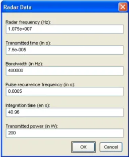
Actual meteorological data were not available, so they were roughly derived from the actual data (observing the orientation and plane of the Bragg lines). IMPORTANCE OF THE SIMULATED DATABASE 123 They were obtained with the same bandwidth (400 kHz), at 3 different frequencies.
INTEREST OF THE SIMULATED DATABASE 123 They have been acquired with the same bandwidth (400 kHz), at 3 different frequencies
136 5.3.2 Method 2: Estimating coherence extent by examining eigenvectors 149 5.4 Application of adaptive filtering to sea echo reduction. To do so, the first step is to develop and test a filtering algorithm on simulated data and then to validate it on real data.
How to reduce ocean clutter?
The objective of this last chapter is to implement an adaptive filtering method for sea echo reduction.
HOW TO REDUCE OCEAN CLUTTER? 127 radar signals interact with selected sea waves. The important sea clutter contribution is
In general, we have more range cells than beams in azimuth, so we will prefer to use adaptive filtering by estimating coherence across range cells. An adaptive filtering method seems to correspond to this problem of reducing coherent signals.
Choice of a signal processing method to reduce sea echoes
METHOD USED TO REDUCE SEA ECHOES: ADAPTIVE FILTERING 129 For a Hermitian matrix, all the eigenvalues are real and two eigenvectors associated with them.
METHOD USED TO REDUCE SEA ECHOES : ADAPTIVE FILTERING 129 For an hermitian matrix, all the eigenvalues are real and two eigenvectors associated to
This is the same comment as in the previous point, the covariance matrix can be estimated simultaneously on several dimensions. RS is the covariance matrix of the signals, σ2 is the white noise variance and I the Nref dimension identity matrix.
METHOD USED TO REDUCE SEA ECHOES : ADAPTIVE FILTERING 131 eigenvalues are given by
23], showed that if noise and interference approximate Gaussian processes, then maximizing the signal-to-noise ratio is equivalent to maximizing the probability of detection. In fact, this is an optimal Neyman-Pearson1 detector for a known signal vector in colored Gaussian noise with a known covariance matrix is linear, i.e., it consists of a linear combination of vector components.
METHOD USED TO REDUCE SEA ECHOES : ADAPTIVE FILTERING 133 and the variance
That is, the convergence to achieve a certain signal-to-noise ratio depends on the adoption criterion. This is the expected loss in power ratio if only K data samples were used to estimate RˆN.
REAL DATA ANALYSIS : ESTIMATION OF COHERENCE 135 5.2.2.2 Consequences of the adaptive filtering
Real data analysis : estimation of coherence
Radar frequency: in function of the carrier frequency, different sea waves will scatter the electromagnetic wave back to produce sea debris. In fact, the frequency domain "correlation" between input and output signals of a system can be defined as the ratio of the correlated cross power (i.e. the cross spectrum) to the uncorrelated cross power.
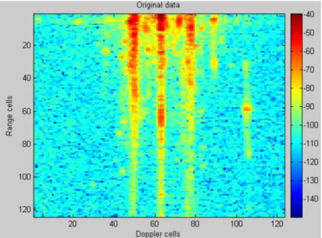
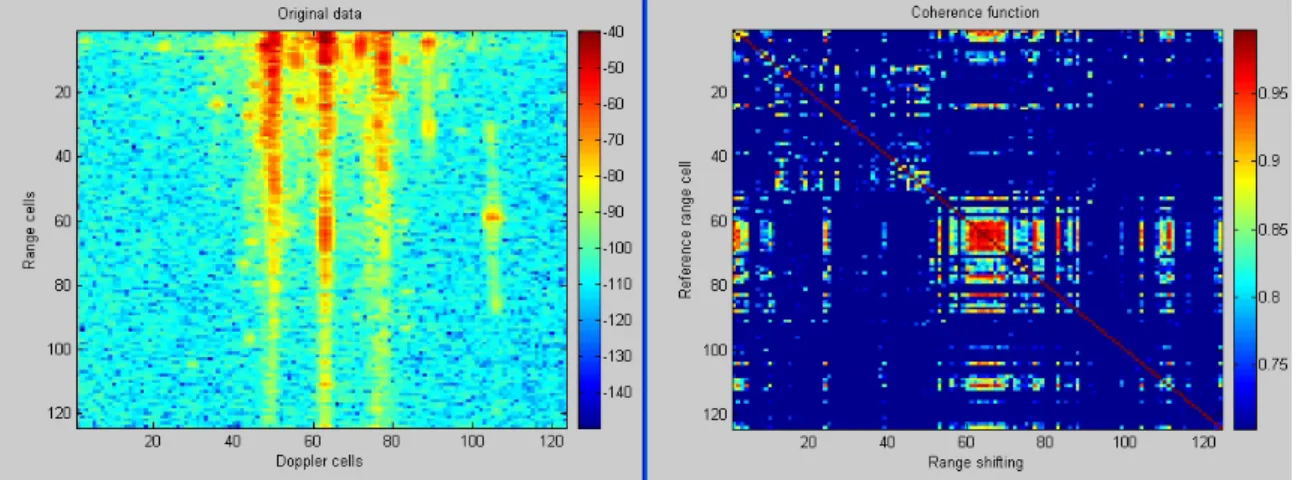
REAL DATA ANALYSIS : ESTIMATION OF COHERENCE 137 In fact, we consider a spectrum at a given range cell k called spectrum k (line vector)
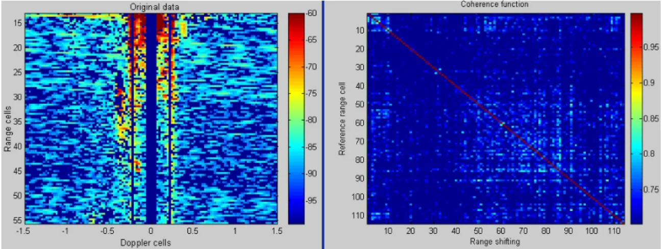
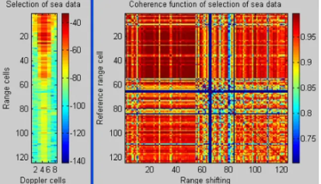
If the spectrum of the series cell 50 is chosen as a reference, the results of the coherence function calculation will be with spectra of all series cells. The Y-abscissa relates to the number of the range cell being referenced, the X-abscissa is the number of the range shift.
REAL DATA ANALYSIS : ESTIMATION OF COHERENCE 139
REAL DATA ANALYSIS : ESTIMATION OF COHERENCE 141 1.4 Coherence of the second order along range cells
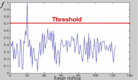
The resulting coherence image is all red, meaning that this Bragg line alone is highly coherent along the entire range cells. Repeating this operation on the positive Bragg line (see Figure 5.12), we notice that the coherence is high except in the zones where the signal-to-noise ratio is not sufficient to distinguish the Bragg line from noise.
REAL DATA ANALYSIS : ESTIMATION OF COHERENCE 143
Then we take more data around this central line, we notice that the coherence decreases (see figure 5.15). When we start to consider Bragg lines, the coherence is not at all good as shown in figures 5.16 to 5.18.
REAL DATA ANALYSIS : ESTIMATION OF COHERENCE 145
REAL DATA ANALYSIS : ESTIMATION OF COHERENCE 147 1.8 Coherence of simulated data
Even if it is not necessary to study the coherence of data along Doppler cells, it can be useful to know, for example, whether first- and second-order Bragg clutter is coherent along Doppler cells or not. The result in Figure 5-24 shows that the coherence along Doppler cells is not good at all.
REAL DATA ANALYSIS : ESTIMATION OF COHERENCE 149 1.11 Conclusions about coherence analysis with the coherence function
With the estimation condition: Mestim ≥ 2.Nref all signals present in the covariance matrix are separated. As a general rule, each signal present in the covariance matrix corresponds to an eigenvector and an eigenvalue.
REAL DATA ANALYSIS : ESTIMATION OF COHERENCE 151 all the correlations have a value comprised between 0 and 1 (both excluding) and the Q
REAL DATA ANALYSIS: COHERENCE ESTIMATION 151 All correlations have a composite value between 0 and 1 (both excluding) and Q. REAL DATA ANALYSIS: COHERENCE ESTIMATION 153 reference eigenvectors are evaluated in the matrix and the first matrix is compared.
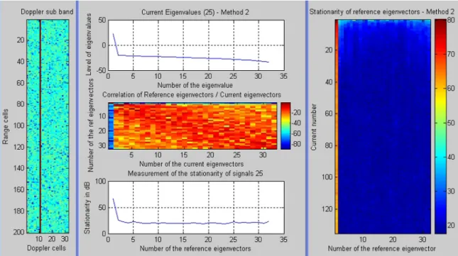
REAL DATA ANALYSIS : ESTIMATION OF COHERENCE 153 reference eigenvectors matrix is estimated on a first portion of signal and then compared
According to this stationarity study (see results on figure 5.28) these interferences can be decomposed into several stationary signals. This means that these jammers can be considered as a coherent source in our filtering algorithm and this is a positive point because they will be rejected as marine debris at the same time.
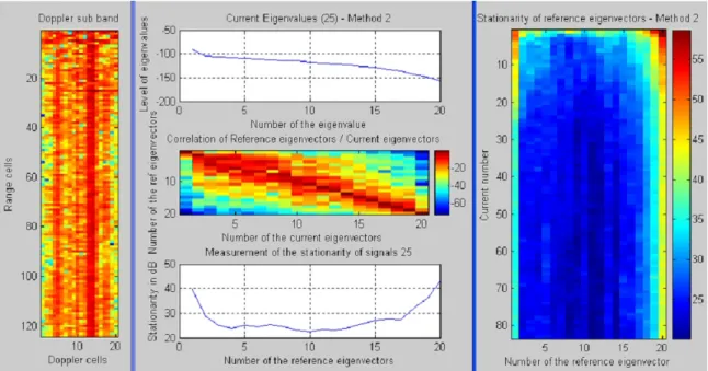
REAL DATA ANALYSIS : ESTIMATION OF COHERENCE 155
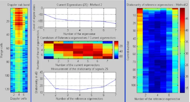
Stationarity of the positive Bragg line (zone 4) Same comments for this fourth zone, the positive Bragg line is selected and the results in Figure 5-31 show that a strong signal is stationary along range cells. According to the results presented in Figure 5-32, the target is not as coherent along range cells.
APPLICATION OF ADAPTIVE FILTERING TO SEA ECHOES REDUCTION157
Application of adaptive filtering to sea echoes reduction
To see if this algorithm is effective, the first step is to test it on simulated data coming from the database. It is very easy to hide a target in sea clutter, at a lower level to see the effect of filtering on the target.
APPLICATION OF ADAPTIVE FILTERING TO SEA ECHOES REDUCTION159 The entered target velocity is very low to be sure that its simulated echo will be hidden
In fact, if we apply the simple algorithm directly to a sample of real data, the result is not good at all (see Figure 5.37, which shows the effect of adaptive filtering on real data). We notice that the center line was reduced, but the filtering did not affect the sea disturbance.
OPTIMIZATION OF THE ALGORITHM ON REAL DATA 161
Optimization of the algorithm on real data