Unité de Recherche : Institut de Recherche en Communication et Cybernétique de Nantes (IRCCyN) Soutenue le 4 décembre 2014. Je tiens à remercier tout particulièrement Agnès Le Roux, Tanguy Lapegue, Axel Grimault, Clément Fauvel, Xin Tang, Thomas Vincent Juliette Medina, et Mi Zhang pour avoir partagé des moments inoubliables avec moi.
Contexte
État de l’art sur les problèmes de localisation intégrant les principes du développement durable 11
Une collaboration entre ces deux communautés sera nécessaire pour résoudre des modèles de localisation étendus, comme des problèmes de routage de localisation par exemple. Une approche hiérarchique consiste à déterminer les variables binaires de localisation à l'aide des opérateurs de l'algorithme LNS, et les variables de flux continu en résolvant un sous-problème à chaque itération.
Optimisation simultanée du coût et de l’impact environnemental
Il en résulte un ensemble de solutions mutuellement non dominées qui constitue l'approximation initiale du front de Pareto. Mais dans tous les cas, on obtient une approximation du front de Pareto qui contient un ensemble de solutions non dominées.
Perspectives de recherche
They call for a reexamination of many supply chain management (SCM) concepts from an environmental and sustainability perspective [Chaabane et al., 2012a, Srivastava, 2007]. As a result, concepts such as green supply chain management, sustainable supply chain management, and reverse logistics have recently attracted many researchers and practitioners.
Solution method
Thesis objectives
We extend the considered supply chain network to a bi-objective model by including a general objective function that measures the environmental impact of emissions. The bi-objective model is made more realistic by the possibility of having different potential technology levels.
Thesis plan
- Delimitations and search for literature
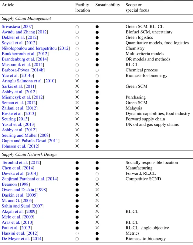
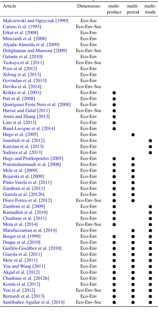
- Position in the literature
- Distribution across the time period and main journals
- The 3 pillars of sustainable development
The start of the time period was chosen so that the Brundtland report from the World Commission on Environment and Development [Burton, 1987] served as a starting point, in the same way as Seuring and Müller[2008] and Chen et al.[2014]. They study the factors that influence location decisions, but these reviews do not review the quantitative models and methods. Devika et al.[2014] is a research paper that contains a literature review section.
Environmental Supply Chain Network Design
LCA based models
In the context of fuel supply chains, cradle-to-grave is called well-to-wheel (WTW). For example, Elia et al.[2011] provides an analysis for hybrid coal, biomass and natural gas to liquids (CBGTL) plants.
![Figure 2.4: Conceptual framework of LCA [ISO, 2006]](https://thumb-eu.123doks.com/thumbv2/1bibliocom/460817.67574/30.892.300.583.149.355/figure-conceptual-framework-of-lca-iso.webp)
Partial assessment of environmental factors
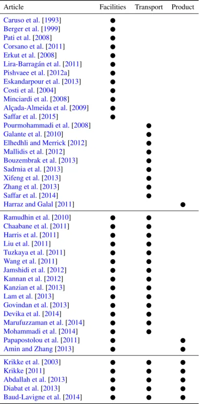
Krikke et al.[2003] propose a mixed-integer linear program (MILP) whose decision variables relate to network design and product design. In Harris et al.[2011], the amount of energy used is a tool to estimate GHG emissions.
Conclusion
2008] measures an unusual material opportunity cost which is the extra expense a firm is willing to pay when it refuses to replace the new material market with an acceptable recycled material. Other criteria are sometimes not detailed, such as the soil-specific technical requirement in Tuzkaya et al.[2011].
Social Supply Chain Network Design
Modeling Approaches
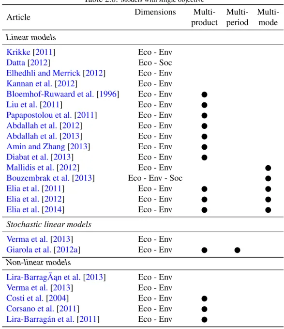
Models with a single objective
In Abdallah et al [2012] and Kannan et al [2012] the objective function is the sum of various logistics costs and an additional term related to CO2 emissions above the amount allocated by the government. The objective function includes the cost of wastewater treatment, while water quality appears as a constraint. Mallidis et al.[2012] propose a model with several objective functions related to the cost and emission of CO2 or particulate matter (fine dust).
Multi-objective models
This is especially true when considering the uncertainties at the level of customer requirements within a strategic planning horizon. 2013] study the effect of demand uncertainty on the economic and environmental performance of supply chains.
Conclusions on modeling
In Guillén-Gosálbez and Grossmann [2010], the value of damage factors is considered as an uncertain parameter, so a probability constraint model is applied to deal with it. As in Guillén-Gosálbez and Grossmann [2009], the stochastic model is converted to a deterministic model to facilitate the solution.
Solution Methods
- Solution methods for models with a single objective
- Solution methods for multi-objective models
- Modeling tools and solvers
- Conclusion
In Kostin et al. [2012] ε-constraint is followed by a strict MILP dimensionality reduction approach based on the definition of δ-error [ Guillén-Gosálbez , 2011b ]. Eskandarpour et al [2013] use a parallel Variable Neighborhood Search (VNS) to solve a multi-objective reverse supply chain planning problem for after-sales services.
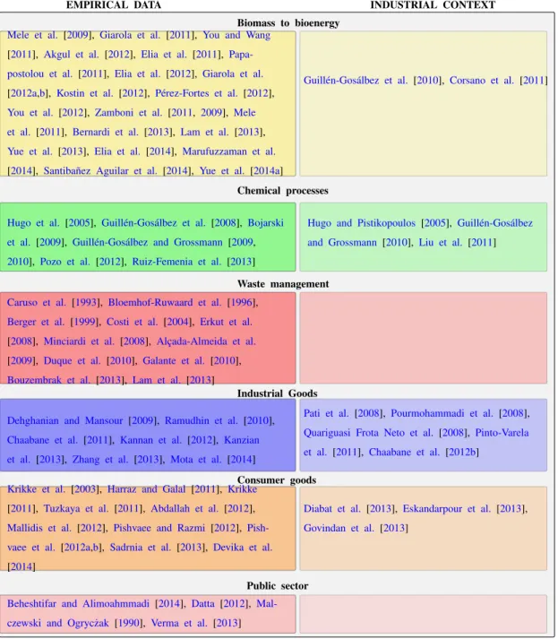
Applications
- Biofuels – bioenergy
- Chemical Processes
- Regional Planning, Waste Management, Public Services
- Industrial goods
- Consumer goods
- Public sector
- Intersectorial analysis
- Conclusion on applications
Berger et al [1999] propose a comprehensive multi-criteria optimization model for comprehensive regional solid waste management planning. Paper: Raw materials such as forests are one of the essential pillars of the paper industry [Pinto-Varela et al., 2011].
Discussion
Summary of findings
As mentioned above, we identified that a large majority of the works focus on the economic and environmental factors. Furthermore, there are a limited number of sub-factors of the three main dimensions considered in published studies. Although uncertainty is often an intrinsic feature of the studied problems, most authors still use deterministic models.
Suggestions for future works
Concluding remarks and research proposed
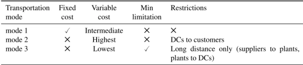
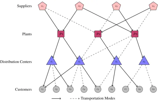
It also integrates advanced decision variables such as the transportation modes between each pair of facilities. Processing costs are variable costs assumed in proportion to the level of activity (i.e. the outgoing flow) of the corresponding facility. At the strategic level, the cost of most modes of transport is assumed to be linear with respect to the quantity of transport.
Data, sets and parameters and variables
Mathematical formulation
Conclusion
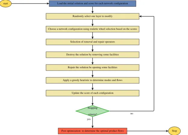
One of the main issues is that there are (Jmax−Jmin)×(Kmax−Kmin) possible network configurations. In general, the main idea of the LNS algorithm in those problems is to remove a number of clients or tasks with a destruction operator and then reinsert them with a repair operator. They take into account several stopping criteria such as the maximum number of iterations and the maximum execution time of the algorithm.
An LNS heuristic for supply chain network design
Removal operators
Vertical cluster removal: the goal is to close a number of plants and GSs that are related to each other, i.e. A first possibility is to randomly close one plant as a seed and then the nearest open DCs. A second possibility is to randomly close one DC as a seed and then the nearest open plants.
Repair operators
Cluster Customers-DC: the idea of this operator is to open DCs near clusters of customers. Therefore, this operator can generate a solution with fewer open facilities than in the target network configuration. Bottom-up flow assignment: this operator is symmetric to the top-down assignment described above.
Removal and repair
Unit cost ratio: this operator favors facilities with high available capacity and lower fixed costs. This operator repairs the broken solution by adding the material flow corresponding to the unsatisfied demand. First we add the product flow from I to J and then from J to K, so we call this top-down flow assignment operator.
Network configuration
Determining transportation modes and product flows
In line 9 of Algorithm2, we apply a greedy heuristic to select the product flows and the transport modes between facilities. We first determine the transport modalities and the product flows between all DCs and customers, which is described in Algorithm3. We then apply the same principle to determine modes of transport and product flows between factories and DCs and between suppliers and DCs.
Conclusion
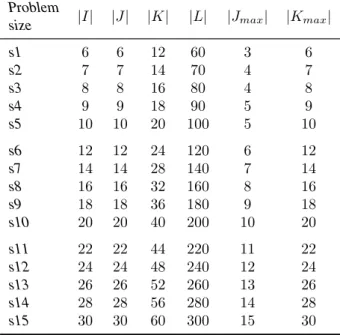
The size of these instances is determined by the number |I| of suppliers, the number |J| of candidate plants, the number |K| of candidate DCs, the number |L| of customers and upper bounds |Jmax| and |Kmax| on the number of plants and DCs that can be opened. Similar to Cordeau et al.[2006], we set the number of potential suppliers and facilities to The goal of generating small test instances is to compare LNS solutions with known optimal solutions obtained with a MILP solver.
Data generation
Generating various patterns of supply chain
The fixed costs of opening facilities vary depending on the prices of the real estate market in each region. The variable transport cost tc1pij on arc (i, j) ∈ A with mode 1 for product p was determined randomly in the interval [0.8,1.2]×tij ×τ, where tij is the distance between the nodes and j, and τ is the parameter representing the costs in every layer of the supply chain. Then the capacity of each DC was chosen randomly with a uniform distribution in the interval[ u.
Conclusion
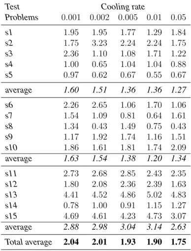
- Cooling rate and initial temperature
- Number of iterations
- Network configuration
- Evaluation of the LNS operators
- Effectiveness of cluster operators
- Heuristic based on cost and depot
- Calculating the product flows with an exact method
- Determining the product flows and transportation modes with an MIP solver
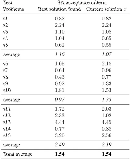
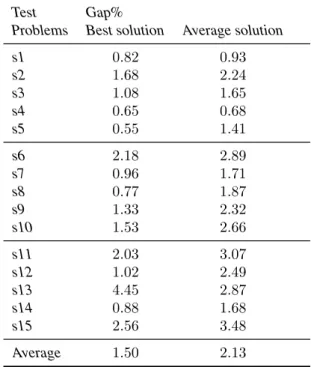
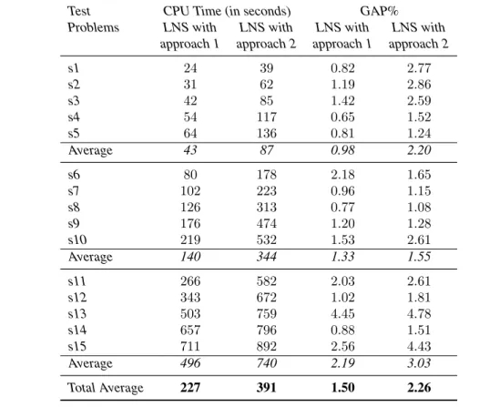
To do this, we consider two approaches: (1) selecting the best solution found at each network configuration as a performance indicator, and (2) calculating the average value of the solutions within each network configuration. Table 6.5 shows the number of visits from each network configuration during the execution of the LNS for a small instance. The first two columns show the CPU time of the LNS heuristic for each approach.
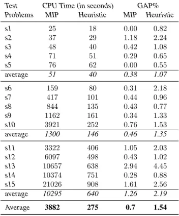
Computational results
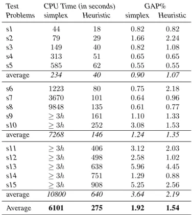
It is worth noting that the best, average, and worst results (columns 5–7, columns 8–10) and the insignificant difference between the results for each pattern are good indicators of the stability of our heuristics. The maximum runtime of the LNS is 923 seconds with an average of 269 seconds, demonstrating that the heuristic is capable of finding good results in an acceptable time. In addition, it can be noted that the CPU time of the LNS is not affected by the data pattern.
Sensitivity analysis
Influence of demand
Influence of varying variable cost on network configuration
Conclusion
As noted in Chapter 2, minimizing network costs is the most common goal in the SCND literature. We believe that CO2 emission is the only environmental impact that is a very popular environmental index and can be easily measured [Wang et al., 2011]. Different types of logistics networks have been used in the related literature, depending on the application or assumptions of the problem.
Problem definition
Data, sets, parameters and variables
Mathematical formulation
Two trends can be recognized in the literature dealing with multi-objective problems: (i) providing at most one trade-off solution in a single run, and (ii) providing multiple trade-off solutions in a single run. Basic definition and metaheuristics related to multi-objective optimization are recalled in sections 8.1 and 8.2. The algorithmic framework of the proposed bi-objective LNS (BOLNS) is presented in section 8.3. Multi-objective optimization algorithms aim to find Pareto-optimal set consisting of several trade-off solutions rather than just one optimal solution [Eberhart et al.,1996].
An overview of recently published metaheuristic for SCND models
In this section we recall the main concepts of multi-objective problems according to Zitzler et al.[2004]. With many multi-objective optimization problems, knowledge of this set helps the decision maker to choose the best compromise solution. Therefore, in what follows, we will assume that the goal of the optimization is to find or approximate the Pareto set.
Algorithmic framework for BOLNS
- Phase I
- Phase II
- Phase III
- Test instances
- Environmental factors
- Fixed and processing costs
Therefore, we intensify the search around every undominated solution of the Pareto set approximation. To do this, we first make a local Pareto set approximation for each non-dominated solution (Rule 2). The local Pareto set approximation is initialized with an undominated solution from the Pareto set approximation (line 3).
Epsilon constraint method
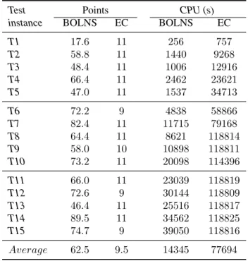
Solving the cost-measure model for 11 different values of ε for environmental impact resulted in having 11 mutually non-dominated solutions including 2 extremes and 9 intermediate non-dominated solutions. However, as instances become larger, finding an approximate Pareto front including Pareto-optimal solutions becomes more difficult. As shown in column 2, the number of non-dominated solutions is less than 11 in some cases.
Parameter Settings
Evaluating the performance of each phase
As stated earlier, due to the optimal value of the product flows, some of the solutions may be dominated by neighboring solutions. Figure 9.7 shows the approximate Pareto front provided by each stage during a run of example T8.
Performance measures
The hypervolume measure
The unary epsilon indicator
The ratio of approximated Pareto front
Computational results
The BOLNS also outperforms the estimated Pareto front of the EC in terms of hypervolume in medium and large instances. Therefore, relative to the trough, the volume of these fronts is naturally larger than the estimated Pareto fronts of the EC. Finally, we assess the ability of the BOLNS to provide good quality ends of the approximate Pareto fronts.
Supply chain topology
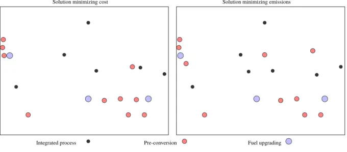
Since the cost objective does not matter for solution C, the maximum allowed number of objects is opened. But unlike solution A, the technology with the lowest fixed cost is used in most facilities in solution A. Table 9.8 shows the distribution of the number of open plants and DCs for each location fixed cost range.
Conclusion
Environmental supply chain network design problems are analyzed with a special emphasis on Life Cycle Assessment (LCA). A multi-objective facility location model for closed-loop supply chain network under uncertain demand and yield. Multi-criteria decision making for the supply chain design: A review with emphasis on sustainable supply chains.
Considering GHG emissions changes the logistics network
Time distribution of reference papers
Distribution of reference papers by journal
Distribution of reference papers with respect to the 3 sustainability dimensions
Conceptual framework of LCA [ISO, 2006]
LCA scopes
Review of industrial applications
The supply chain considered
Example of supply chain pattern 2
Example of supply chain pattern 3
Example of supply chain pattern 4
Number of best solutions found within process iterations
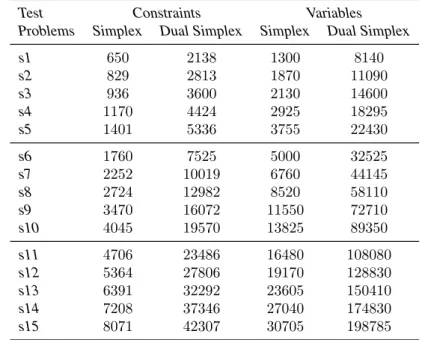
Comparing the CPU time of simplex and dual simplex algorithms
Example of LNS iterations (Test set s15, pattern 4)
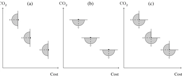
Relevant portions of solution space. (a) Relevant portion of solution space in favor of cost
Updating Pareto set approximation in phase II. (a) Starting set of solutions. (b) Neighbors
Influence of phase III on the Pareto set approximation. (a) Pareto set approximation at the
Number of new non-dominated solutions found within phase II
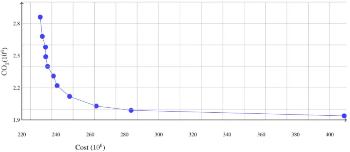
Comparison of the approximated Pareto fronts for instance T10
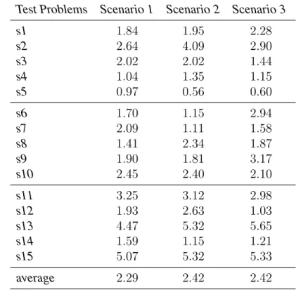
CPU time consumed by each scenario
Impact of the frequency of phase III (instance T10)
CPU time consumed by each scenario during the tuning of phase III
Mutually non-dominated solutions found by each phase of the BOLNS for test instance T8 133
Comparison of the Pareto fronts for instance T3
Comparison of the Pareto fronts for instance T8
Comparison of the Pareto fronts for instance T13
Approximated Pareto front for instance T4
Supply chain topology in solution A