Can Uncertainty Justify Overlapping Policy Instruments to Mitigate Emissions ?

It has been known since Weitzman (1974) that under uncertainty the relative slope of the marginal cost and marginal benefit curves is crucial for choosing between a price instrument (e.g. a carbon tax) and a quantity instrument (e.g. a cap-and-trade -system). , such as the EU ETS). More specifically, in the simplest form of Weitzman's (1974) model, the quantity instrument should be chosen if the marginal benefit curve is steeper than the marginal abatement cost curve, while the price instrument should be chosen if the marginal abatement cost curve is steeper. If the marginal benefit curve is completely flat, a tax (set at the expected marginal benefit) is the first best tool.

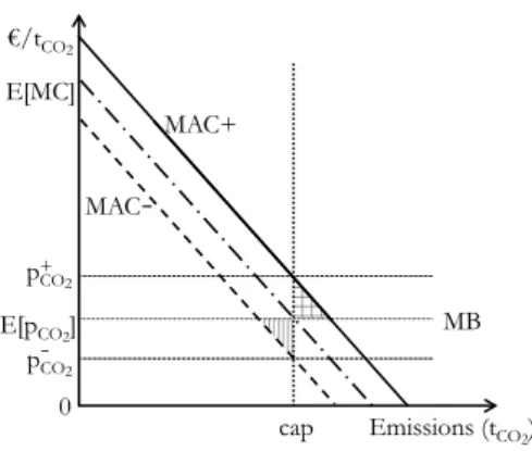
Let us assume that the Marginal Benefit MB is known with certainty and is completely flat. Let us further assume that the marginal abatement cost curve is uncertain and can take two values, MAC+ and MAC-3, with equal probability. In Figure 1a, with a low uncertainty, the policy maker would set the optimal ceiling at the intersection of the marginal benefit and the expected marginal abatement cost curve (the dashed line).

They show that while equivalence prevails with additive uncertainty (a shift of the marginal abatement cost curve as in Weitzman's original paper), it does not occur under multiplicative uncertainty (a change in the slope of the marginal abatement cost curve). Conversely, in Figure 1b, which has a large uncertainty, setting the optimal ceiling at the intersection of the marginal benefit and the expected marginal abatement cost curve (vertical dashed line) does not minimize the expected cost: such a ceiling would not be binding in the MAC. - state, but it would incur a significant cost, both in the MAC mode (region with vertical lines) and in the MAC+ mode (region with squares). Note in Figure 1c that in the MAC+ condition the marginal abatement cost is equal to the marginal benefit; therefore the welfare loss from a marginal additional effort would only be of the second order.

Conversely, in the low-cost state, the marginal cost of abatement is below the marginal benefit; therefore the welfare gain from an additional marginal effort would be first order.

Analytical framework and equations

A better solution (Figure 1c) is to set a milder limit that equalizes the marginal abatement costs and benefits only in the MAC+ state: the additional costs compared to the pricing instrument would then be zero in the MAC+ state, while these would still be equal to the area of ​​vertical lines in the MAC state. Having explained the intuition of our main results, we now turn to presenting the analytical model. To explore in more detail the implications for the energy sector of possible zero CO2 emissions.

This uncertainty may be related to the uncertain marginal cost of abatement from the previous section, as higher/lower energy demand will result in higher/lower abatement effort for a given emission cap and thus higher/lower marginal cost. The following subsections highlight some key analytical results based on the assumptions presented in the previous section. They refer, for example, to investments that enable coal-fired power plants to handle a certain proportion of biomass, CCS investments or purchases of rights in the Clean Development Mechanism (CDM) market.

Medιf andιr function the intercepts (iota-like intercept) of the fossil fuel and REP marginal supply and σr the slope (sigma-like slope) of the REP marginal supply function, respectively. We define a linear downward power demand functiond(·) (withd0(·)<0) whose intercept depends on the state of the world. The equilibrium conditions on the electricity and emissions market thus depend on the state of the world.

In every country of the world, the supply of electricity must meet the demand in the electricity market. In a high-demand world, total emissions cannot be higher than the upper limit Ω, so the price of CO2 is strictly positive. In the low-demand state, we assume that the cap is non-binding, so the CO2 price is zero.

The values ​​of the market variables (p, f, r, a, φ) as a function of policy instruments are found by solving the system of equations (2) to (6). After replacing the market variables in the expected welfare function (7) with the response functions arising from the producer problem, we maximize expected welfare. The first-order conditions give the optimal levels of the policy instruments in all states (ρ? and Ω?).

Social optimum when the CO 2 price is nil in the low demand state

When the CO2 price is zero in the low-demand world, the expected carbon price and the renewable subsidy equivalent in e/tCO2 are such that a linear combination of the two equals the marginal benefit. The simple intuition behind this result is that since the expected CO2 price is below the marginal benefits, the additional instrument, e.g.

Expected emissions with various instrument mixes

The simple intuition behind this result is that, since the expected CO2 price is below the marginal benefits, the additional instrument, e.g. the REP grant is also used to reduce emissions.

Boundary condition for having a nil CO 2 price in the low demand state of the world

Variables’ elasticity with respect to parameters

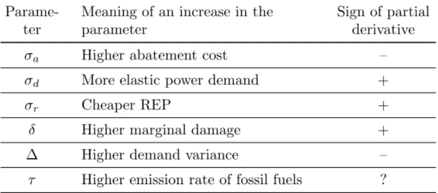
1;0[ indicates an elasticity between 0 and -1; ]0;1[ indicates an elasticity between 0 and 1; + or – indicate a positive or negative elasticity, respectively;. Table 4 shows the sign of the change of the optimal levels of the policy instruments when different parameters change6. A positive elasticity indicates a positive change when a parameter increases, and an absolute elasticity less than one indicates that a 1% change in that parameter will cause less than a 1% change in the variable.

We see that the elasticityρ with respect to σa and σ is positive but less than 1, with respect to σdit it is negative but less than one, and the elasticity with respect to δ is 1. The interpretation of this result is simple: more REPs should be installed when environment Ecological damage is higher when REPs are cheaper and when there are other ways to reduce emissions, i.e. Similarly, higher abatement costs naturally lead to a less stringent cap on emissions Ω, while higher marginal damage and more elastic power demand (meaning higher energy savings for a given change in electricity price) result in a tighter cap.

The impact of a cheaper REP on the optimal limit is ambiguous: on the one hand, it reduces the overall cost of emissions reduction, leading to a stricter limit, but on the other hand it leads to an increase in the use of the instrument another of politics. subsidy, which undermines the importance of the emissions cap. Therefore, the considered parameters increase the amount of REPr− and decrease the amount of fossil fuel electricityf− when increasing the REP subsidy. In the + state, as might be expected, more abatement a and a higher CO2 price φ+ are caused by a lower abatement cost, a more elastic energy demand, more expensive REP, and a higher damage marginal.

In addition, a higher electricity price is triggered by higher marginal damage, more expensive REP, more elastic energy demand and, even more surprisingly, lower abatement costs. The explanation is that lower abatement costs mean a stricter target (Table 4), which in turn increases the price of electricity in the country. In the + state, changes in energy production follow changes in the CO2priceφ+: lower abatement costs, higher marginal damages, and more elastic energy demand raise the price of CO2, which in turn reduces the relative competitiveness of fossil fuels.

In the state - the CO2 price is zero and changes are more sensitive to the REP subsidy: higher abatement costs, higher marginal damages and a more elastic energy demand increase the optimal REP subsidy, which increases the relative competitiveness of REP. Comparing Table 4 and Table 3 finally shows that the carbon price and the REP subsidy change in opposite directions (except when the marginal damage changes). When the carbon price is zero in the world's low-demand state, the mitigation efforts induced by the carbon price are no longer sufficient.

Modified model

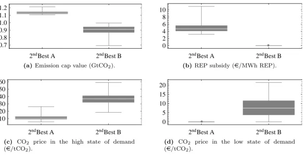
In the second category (subsequently called 2ndBest A), the CO2 price is zero in the low demand state and the renewable subsidy is strictly positive.

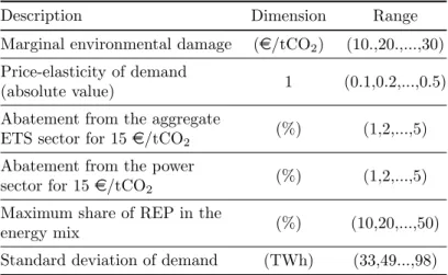
Data and assumptions for calibration

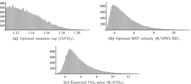
Optimal policy instruments and CO 2 price levels

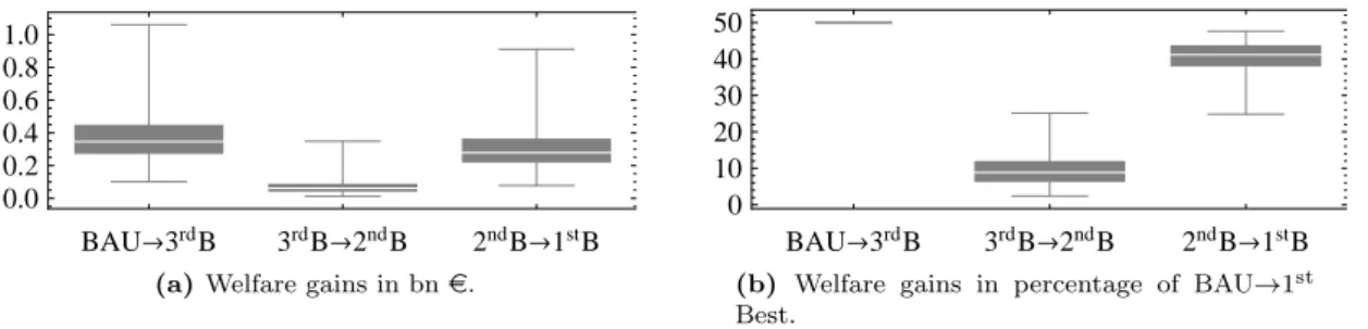
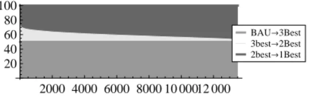
Expected welfare gains from adding a REP subsidy

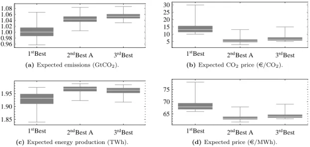
Expected emissions, productions and prices with various instrument mixes

Shift in the optimal emission cap and CO 2 price

6d, there is a strictly positive subsidy (2nd best scenario A in Fig. 6b) and the price of CO2 in a country with high global demand falls compared to 2nd best scenario B (Fig. 6c). We bring a new contribution to the analysis of the coexistence of several policy instruments to cover the same emission sources. They notably highlight the possibility of corner solutions (in this case zero CO2 pricing) when comparing policy instruments and policy packages.

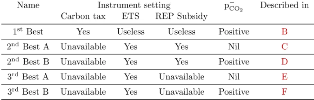
Our results are based on the assumption that the risk of the CO2 price falling to zero cannot be ruled out. Directive 2009/125/EC of the European Parliament and of the Council of 21 October 2009 establishing a framework for setting ecodesign requirements for energy-related products. A Description of the types of models and instrument settings used in the analytical and numerical results.

3. Best B Not available Yes Not available Positive F Table 7: Description of model types and instrument settings. The detailed description of the model framework and the optimal solution calculated using Mathematica are given in the following appendices. Show the framework and the optimal solution for the model used in the numerical part, with setting 2. Best A.

C Second best A settings: model with ETS, REP subsidy and a zero CO2 price in the low demand state. Solving the producer's profit maximization problem gives the producer's response functions, depending on the level of policy instruments and the state of the world. Solving the regulator's welfare maximization problem by knowing all feedback functions yields the optimal level of policy instruments.

D Second Best B setting: model with ETS, REP subsidy and a strictly positive CO2 price in the low demand condition. We have assumed throughout this paper that the carbon price is zero in the low demand state of the world. E Third Best A setting: model with only ETS and a zero CO2 price in the low demand condition.

F Third best setting B: ETS-only model and positive CO2 price at low demand. G Model with permits from non-energy ETS sectors and zero CO2 price at low demand.