Zheng Chen

Dans cette thèse nous nous intéressons à la minimisation de la norme L1 du contrôle pour le problème circulaire contraint à trois corps. C'est exactement la condition que l'on peut vérifier numériquement en calculant ces champs de Jacobi (voir par exemple [10,18]).

Definitions and notations

• Circular restricted three-body problem
• Propulsion control systems
• Controlled equation for the CRTBP
• Dynamics
• L 1 -minimization

To address this problem, the controllability of the motion of a satellite in the two-body problem (µ“0 or 1) with a low-thrust control system is defined in Chapter 2. If m :“ m3{m˚ is the nondimensional mass of the spacecraft cosmic, the non-dimensional state x P Rn (n “ 7) for the movement of the satellite consists of ngar, v and m.

Pontryagin Maximum Principle

Let us denote by Hpxp¨q,pp¨qq on r0, tfs the maximized Hamiltonian of extremalpxp¨q,pp¨qqonr0, tfs. If the switching function H1 has either no or only isolated zeros along an extremalpxp¨q,pp¨qqonr0, tfs, this extremal is called a nonsingular.

Singular solutions

Along the non-singular extremalpxp¨q,pp¨qqonr0, tfs, the arc on the finite interval rt1, tfs Är0, tfswitht1 † t2 is called the maximum thrust (or combustion) arc if ⇢“ 1, otherwise it is called the zero arc. thrust (or coastal) bow. Given the extremepxp¨q,pp¨qqonr0, tfs, if H1pxp¨q,pp¨qq ”0 holds on the finite interval rt1, t2sÑr0, tfswitht1 †t2, the arc nart1, t2 is called singular.

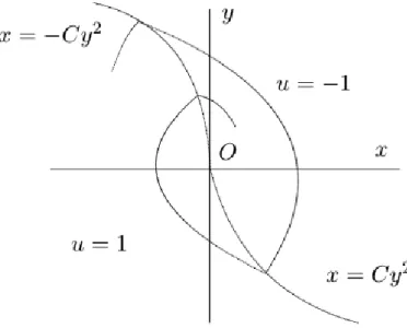
Fuller (or chattering) phenomena

The choice of pz,wqis is not unique and eq. 1.17) is henceforth called the semi-canonical form of the Hamiltonian system of Eq. Note that the Hamiltonian system Eq. 1.19) has an infinite number of switching times in a finite time interval (see the typical picture for the Fuller phenomenon in Fig. 1.2).

Computational method

Contributions of the PhD

Controllability

Sufficient optimality conditions

Then, checking a second order sufficient condition on this auxiliary problem turns out to be sufficient to ensure strong local optimality of the bang-bang controls. In Chapter 4, the extra condition related to the geometry of the target manifold and the Jacobi fields is established.

Neighboring optimal feedback control

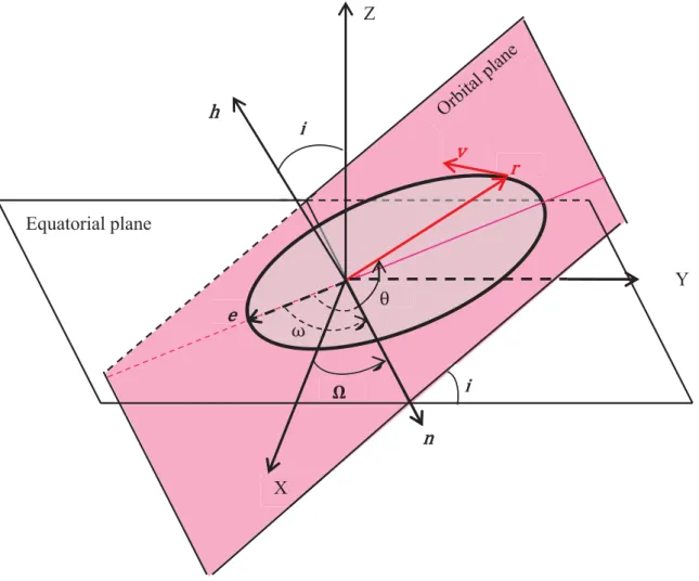
Based on this variational idea, a growing number of papers have been published (see, e.g., and references therein) on the topic of NOG for orbital transfer problems. A common example of the two-body problem is the motion of an artificial body, i.e., spacecraft or satellite, around the Earth (see Fig. 2.1).

Definitions and notations

• Dynamics for controlled two-body problem
• Study of the drift vector field in Y
• Admissible controlled trajectory of ⌃ sat
• Controlled problems in A

We say rppyq and rapyq are the perigee and apogee distances of the orbit y onr0, tppyqs if epyq ‰ 0. For each initial point xi “ pyi, use miq P YrˆR˚`and measurable control function ⌧p¨q assuming values ​​in B⌧max we pt ,⌧ptq,xiq to denote the constraint to R` of the solution of ⌃sat.

Prerequisite for controllability

To study controllability, it is necessary to first show that the allowable region A is a connected subset of P. The allowable region A is an arc-connected subset of P, i.e. for every initial point yi P and every end point yf PA there exists a continuous path yp¨q:r0,1s ÑA, fiÑyp q such that yp0q “ yi, andyp1q “ yf.

Controllability for OTP

Since the subset P` is path connected, as shown by Theorem 2.3, it follows that two different vertices yiandyf in P` are connected by a pathy:r0,1s ÑP`, fiÑyp q such that yp0q “yiandyp1q “yf.

Controllability for OIP

It remains to determine ⌧max so that prptq,vptqqi is part of an admissible controlled trajectory of the system⌃". The limiting value ⌧max can be calculated by combining a shooting method and a halving method as described in section 2.6.

Controllability for DOP

Numerical Examples

A numerical example for OIP

Given each initial toppyi, miq P´ˆR˚`in⌧max °0, the optimal control problem for the OIP consists of pointing the satellite past. p¨q PB⌧max in the time intervalur0, tfsÄI along the system⌃sat such that along the controlled trajectory prptq,vptq, mptqq “ pt,⌧ptq,yi, miq time tf ° 0 is the first occurrence for krptfqk“rpprptfq ,vptfqq, ie .,krptqk°rpprptq,vptqqonr0, tfq, and that rpprptfq,vptfqq is maximized, ie. the cost functional is. 2.20) Let °0 be the optimal final OCP time for OIP and letpryptq,mrptqq “ pt,⌧rptq,yi, miq onr0,rtfs optimal controlled trajectory with associated optimal control⌧rptq PB⌧max. Therefore, the limit value ⌧max in Corollary 2.2 is determined only by k ri k, k vi k and the flight path angle ⌘i P r´⇡{2,⇡{2s, i.e. the angle between the velocity vector vi and the local horizontal plane defined by.

A numerical example for DOP

Conclusion

Remember that the drift vector fieldf0in Eq. 1.4) for CRTBP (µP p0,1q) is recurrent2 in a suitable subregion X of the state space. Although maximizing the finite mass no longer makes sense for the constant mass model (“ 0), the Lagrangian costs in Eq.

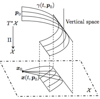
Parameterized family of extremals

The first-order necessary conditions formulated by the Pontryagin Maximum Principle in Section 1.2 can be applied directly. In this chapter we assume that the non-singular extremalpxp¨q,pp¨qq P T˚X at r0,tf is computed from Pontryagin's maximum principle and we say that it is the reference extremal.

No-fold conditions for the projection of F

By restricting the subset P0 if necessary, Fatti's projection ⇧t is a dipheomorphism (a folding singularity, respectively) if the two vectors T´i and T`i point to the same side (the two different sides, respectively) of the link surface ⇧tp⇥ iq(see Fig.3.2). Accordingly, one is immediately told that the projection ⇧tofF aroundti is a diffeomorphism if. and it is a folding singularity if .

Sufficient conditions for strong local optimality

Restricting ourselves to a compact neighborhood of the graph vanz, one can assume that ⇧ induces a homeomorphism on its image. Then set "°0; as a result of the previous discussion, there exists xrof classC1 with the same endpoints as xen whose graph only has isolated contacts with ⇧tp⇥1qsuch.

Numerical examples for problems with fixed endpoints

Case A

The value of the determinant of the Jacobian fields along the extremum is plotted against time. The first conjugate point occurs at att1c «171.20 h°tf; optimality of the reference extremal at r0, tfsfollows.

Case B

The value of the determinant of Jacobi fields along the extremal is plotted against time (details on the right subgraph). The value of the determinant of Jacobi fields along the extrema is plotted against time on the upper left subgraph.

Conclusion

Given a fixed final timef °0, an extremal trajectoryxp¨q PX associated with the extremal control up¨q “ p⇢p¨q,!p¨qqinU onr0, tfsis said to be a weak-local optimum inL8 topology (resp. a strong-local optimum in C0 topology) if there exists an open neighborhoodWu ÑU ofup¨qinL8 topology (resp. an open neighborhoodWx ÑX ofxp¨qinC0 topology) such that for every admissible controlled trajectoryxp¨ q ıxp¨qinX associated with the measurable controlup¨q “ p⇢p¨q,!p¨qqinWu. We say it is a strictly weak-local (resp. strong-local) optimum if the strict inequality holds.

Variation of the Poincaré-Cartan form on M

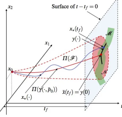
Let us first prove that, under the hypotheses of this statement, Eq. 4.3) is a sufficient condition for the strict strong-local optimality. Since the trajectory x˚p¨qon r0, tfs has the same endpoints with the extremal trajectory xp¨,p0p⇠qq “ ⇧p p¨,p0p⇠qqq onr0, tfs, according to Theorem 3.1, one obtains.

Verifiable condition

Substitute this equation into Eq. 4.12) Since the matrixBxptf,p0p⇠qq{Bp0 is non-singular if condition 3.1 is satisfied, we have.

Numerical implementation for sufficient conditions

Note that the matrix C can be calculated by a simple Gram-Schmidt process when the explicit expression for the matrix d pxptfqq is derived. See Appendix C for the numerical procedure for calculating the matrices Bxp¨,p0q{Bp0 andBpTp¨,p0q{Bp0 onr0, tfs.).

Numerical example for problems with variable target

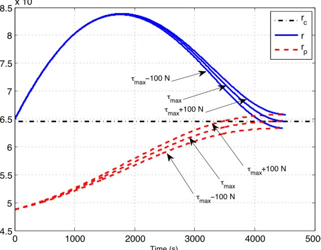
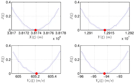
We seek a zero of the shooting function corresponding to a two-point boundary value problem [68]. Fig. 4.2 illustrates the (non-dimensional) profile of the position vector r along the calculated extreme trajectory.

Conclusion

Indeed, the adjacent optimal optimal feedback control is one of the most important practical applications of the optimal control theory (see, for example, [82, Chapter 5]). As for the bang-bang case, the adjacent optimal control consists not only of thrust direction correction, but also of switching times.

Neighboring extremals

Parameterization of neighboring extremals

Given the nominal extremalpxp¨q,pp¨qqonr0, tfs, we denote by Fq “ pt,xptq,pptqq PRˆT˚X |pxptq,pptqq “ pt,qq, tP r0, tfs, qPFpNq( the q-parameter family of neighboring extremals the nominal Recall that the presence of adjacent extremals around the nominal is a prerequisite for constructing the adjacent optimal feedback control (see e.g.

Existence conditions for neighboring extremals

In accordance with the technique for determining kink-free conditions in Chapter 3, we immediately see that the projection ⇧ of Fq is no longer a diffeomorphism if qptq “ 0 for t P pti, ti`1q or qpti´q qpti`q †0fori k . Recall that the classical variational method states that there are no adjacent extrema if qptq “ 0, because the gain matrix explodes in this case (see e.g. [16]).

Neighboring optimal feedback control law

Neighboring optimal feedback on switching times

For every sufficiently small xen every time0 P r0, tfq, one has the following the Taylor expansion. It is clear that xi is the first-order term of the Taylor series of xpti,q˚q ´xptiq.

Neighboring optimal feedback on thrust direction

Numerical implementation

Differential equations

Once the final conditions are given, one can use Eq. 5.11) to calculate the two matricesBxp¨,qq{BqandBpp¨,qq{Bqon the entire intervalrt0, tfs. In the next paragraph, the procedure for calculating the values ​​of the final matrices Bxptf,qq{Bq and Bpptf,qq{Bq will be presented.

Final conditions

Given the r matrix pxptf,qqq, we can compute the full-rank matrix Bxptf,qq{Bq1 by Gram-Schmidt orthogonalization. All necessary quantities to calculate the final conditions are now available zal †. Therefore, we can calculate the gain matrix S by integrating Eq. 5.10) from the above conditions backward between switching times and using Eq. 5.11) to update the boundary condition at each switch.

Riccati differential equation

Substituting this equation into Eq. Given a nonsingular matrix A P Rnˆn and two vectors b P Rn and c P Rn, if the matrix A`bcT is nonsingular, the equation Thus, if the matrixBxpti`,qq{Bq is nonsingular, considering Eq. Bqpti`,qq ` ⇢if1pxptiq,!ptiqqdtipqq dq. 5.21).

Numerical examples for neighboring optimal control

Case A: Constant mass model

Case B: Varying mass model

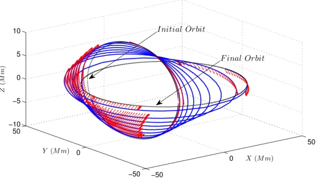
Note that the perturbations on the initial mass are not taken into account, since the corresponding perturbations are equivalent to those on the thrust magnitude or on the acceleration. 5.9–5.11 depict the time evolutions of the errors on semi-major axis, inclination and eccentricity, respectively, showing that the corresponding errors tend to zero at the final time.

Conclusion

Research summary

Since these three conditions are related to Jacobi fields, the numerical test of sufficient conditions eventually turns into the calculation of Jacobi fields. The last part of the research is aimed at establishing an adjacent optimal feedback control law for L1-minimization (cf. Chapter 5).

Future directions

The literature on sufficient conditions of optimality for optimal control problems with state space constraints is limited. A natural extension of this work would be to create such conditions for the optimal path constraint control problems.