In this thesis, we investigate the effectiveness of using Hadoop MapReduce join algorithms to solve Constraint Satisfaction Problems. We start by presenting the Map Reduce framework and continue with a brief summary of the CSPs. We exploit the fact that CSPs and database techniques overlap by modeling a CSP as a database schema.
We describe some of the merging algorithms and then use the above scheme as input to them. Some modifications and preprocessing are made to these algorithms to support the specification of CSPs as joins. Finally we use them to perform a series of experiments and conclude that it is not effective to use the map-reduce framework for CSPs.
INTRODUCTION
MAPREDUCE AND HADOOP
- What is MapReduce
- MapReduce Execution Overview
- MapReduce Example
- Hadoop and HDFS
- What is Hadoop
- HDFS
- The Hadoop Cluster
- Mapper
- Reducer
- Combiner
- Input Split and Input Format
- Shuffle Phase
- Job
It parses key/value pairs out of the input data and sends each pair to the user. In Hadoop terms, these key/value pairs refer to the offset of the current line read from the beginning of the file/the entire line in String form. The default partitioning feature can be overridden by the user to allow custom partitioning. The locations of these cached pairs on the local disk are sent back to the master, which is responsible for forwarding these locations to the reduced workers.
When a reduce worker is notified of these locations by the master, it uses remote procedure calls to read the buffered data from the map workers' local disks. When a reducer has read all the intermediate data, it sorts it by the intermediate keys, grouping all instances of the same key. The output of the Reduce function is added to a final output file for this reduce partition.
Numbers that do not belong to any of the previous sets list them as Res. The mapper class [15] is one of the two classes that the user almost always overrides to perform an MR process. It is important not to confuse the mapping task with the mapping function of the mapper.
The first is a process that executes the entire mapper class, the second is a method of the mapper class. In addition, there is the setup method which is called once before the iteration of map function, usually to perform pre-processing. There is also the cleanup method that is called after the iteration of the map function.
Again, there is also the setup and cleanup methods for the reducer, which the user can override for their own preferences. These methods are called in the run method of the reducer before and after the reducer function in the same way as the mapper. For this, its key/value input types must match the key/value output types of the mapper and its key/value output types to the reducer input types.
The input format is also responsible for providing a RecordReader implementation, which is used to convert the byte-oriented view of the input partition to a record-oriented view. One of the advantages of the task class is that it can create user-defined parameters with the help of the configuration class and pass them to the mappers and reducers.
![Figure 1 - Execution overview [2]](https://thumb-eu.123doks.com/thumbv2/pdfplayerco/312649.45296/15.892.198.767.159.582/figure-1-execution-overview-2.webp)
CONSTRAINT SATISFACTION PROBLEMS
- Definition
- CSP Example
- Solving a CSP
- Modeling a Join as a CSP
Any other way of placing the queens leads to conflict with the constraints of the problem. To model the above problem according to our CSP definition, we define the 4 queens as the 4-tuple of the variables V= {Q1, Q2, Q3, Q4} – one queen for each row. The number of constraints is the number of unique queen pairs, because the values each queen takes is affected by where the other queens are placed.
One of the two classes of strategies for solving constraint satisfaction problems are the systematic search strategies [10]. The other are the repair strategies, but we will focus on the first one in this article. If a value we just assigned doesn't violate any of the constraints, we continue with the.
But if it violates one of the constraints, we choose another value until we choose a valid one. This is the simplest form of the process, known as backtracking, and continues until all possible combinations of values have been selected if all solutions to the problem are to be found. All of the above is the basic idea behind the pre-check strategy [12], which of course can get much more complicated.
Remember that when using the check-ahead strategy described above, we are essentially shrinking the variable domain during the execution of the algorithm, so the first failure works very well for the check-ahead. However, since we refer to equivalent joins, one variable corresponds to all attributes with the same name, regardless of the relationship to which they belong. For example, if we have relations A, B and attributes A.x, B.x, these two attributes represent the same CSP variable.
Second, the domains Di of the variables Vi are represented by the domains of the database schema attributes. In equi-joins, the domain of an attribute is a subset of the domain of the CSP variable to which it corresponds, and the union of the domains of all attributes corresponding to the same CSP variable is equal to the domain of that variable. The subset Sj of variables V is represented by the attributes of the database relationship, and the relationship RSj essentially consists of the tuples in the relationship that are produced by a subset of the Cartesian product of the domains of the attributes of the relationship.

JOIN ALGORITHMS IN MAPREDUCE
- Headers and Join key
- Repartition Join
- Semi Join
- The Algorithm
- Distributed Cache
- The Mapper
- The Reducer
- An Alternative Approach
- Map Side Join
- The Algorithm
- Optimizations
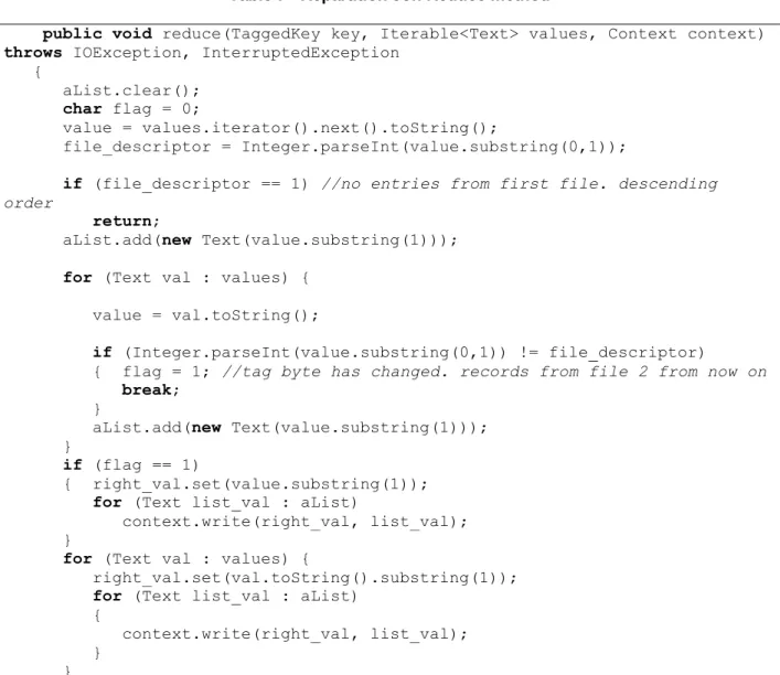
We keep the header of the first file unchanged and bind it to the unique columns that only appear in the second file. At the beginning we put the join key and in the middle the values of the unique columns of the first file. In the reducer all values of the same join key are grouped together by the Joining Grouping Comparator.
We check the values of the iterables one by one and add them to a list. The input of the next job is the output of the previous one plus a file of our choosing. In the first stage we choose the smaller of the two files and use it as input for our work.
In the second job, we cache the output of the previous job in the distributed cache and use another file as input. The broadcast merge selects the smaller of the two files and places it in the distributed cache. In our example, the two files are the output of the second stage and the first file (which was used as input in the first stage).
We associate each record returned by the structure with the current line in the input file. String new_header = StringManipulation.new_header(header2, keys[3], separator); //the header of the output file. We start with the setup method, where we get the name of the input file from the input split.
We use this to get the index of the current column name in this input file. For each record in the cache file, we use the values of the global columns as the key for our structure and the entire record as the value. In the mapper's map function, we split each line in the current column using the index.
One of the two files is always the output from the previous map job. Remember that the number of output partitions is the number of reducers used and.
EXPERIMENTS
N Queens
Spatially Balance Latin Squares
CONCLUSION