The created database will then be used in Design Studio and loaded into a Data Model Project ( OLAP. After working on the Data Model Project, we will build a data warehousing application that will be deployed on the Websphere Application server.
Presentation of the A.T.E.I
Goals of the project
Technical Environment and used tools
DB2 Data Warehouse Edition V9.1.1 overview
Introduction
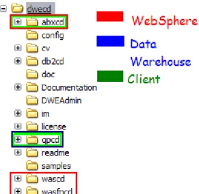
Provided products
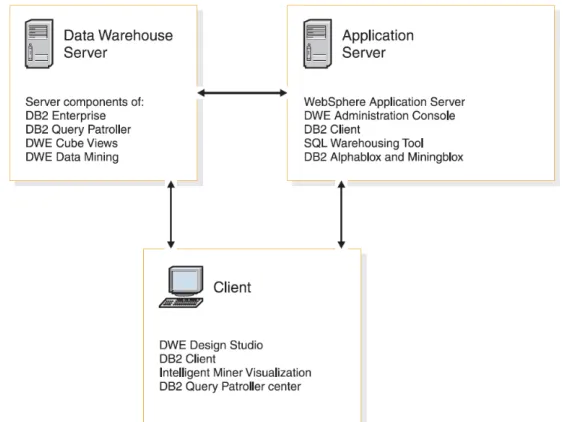
DB2 DWE architecture
DB2 DWE components
DB2 Enterprise Server Edition is a multi-user relational database management system specifically tailored for managing data warehouses. This version is specially tuned for data warehouse management due to features like "data compression features" that reduce the need for large disk space.
The fictional company
Presentation of the JK Superstore
Understanding of the need of the company
The sample database
The current technical situation of the company
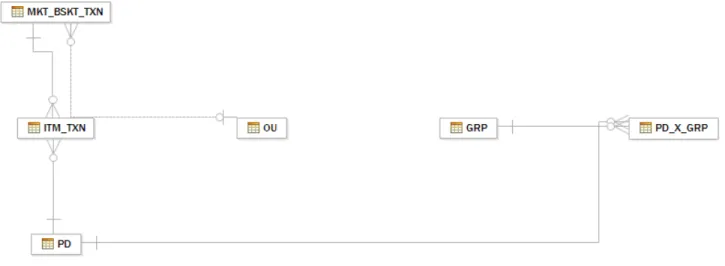
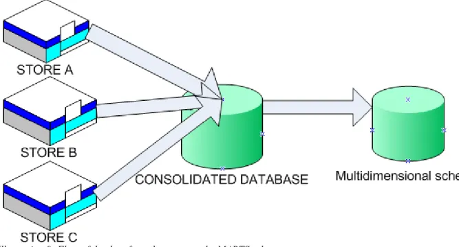
The Data Warehouse Schema
The Organizational Unit (OU) table is loaded with the various stores belonging to JK Super Store. The Product Table (PD) is designed to contain the various products offered by JK Super Store.
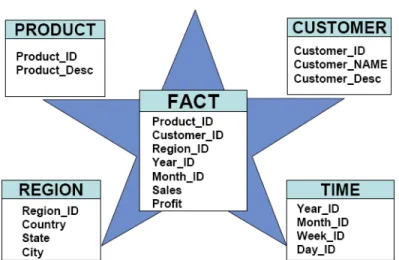
The Data Marts Schema
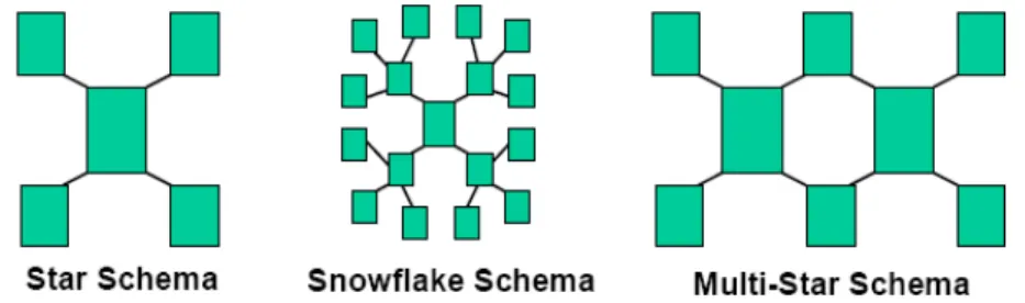
- What is a dimensional model
- The JK-Superstore Marts
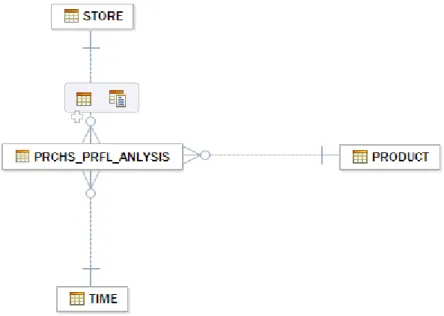
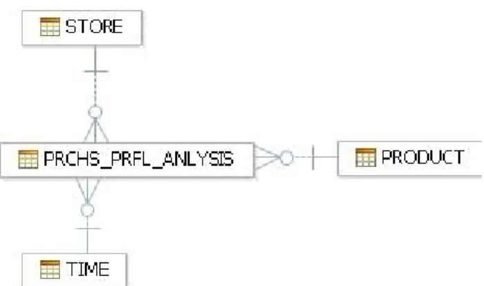
This schema contains the aggregated data that will be used to make analyzes of the sales and prices of JK Superstore. The three dimension tables are the TIME, STORE and PRODUCT and the fact table is called PRCHS_PRFL_ANALYSIS.
Prerequisites before starting with tutorials
How to install DB2 DWE Edition 9.1.1
Creation of the database
Code: Part of .bat file that creates DWE schema and MARTS -- Creating DWE schema tables. Add stored functions, to be used by MARTS schema db2 -tvf sqw\dwesamp_marts_func.sql.
The Eclipse based Integrated Development Environment
Introduction to the Design
Projects in Design Studio
Global aim of these tutorials
The tutorials and their goals
Introduction and prerequisites
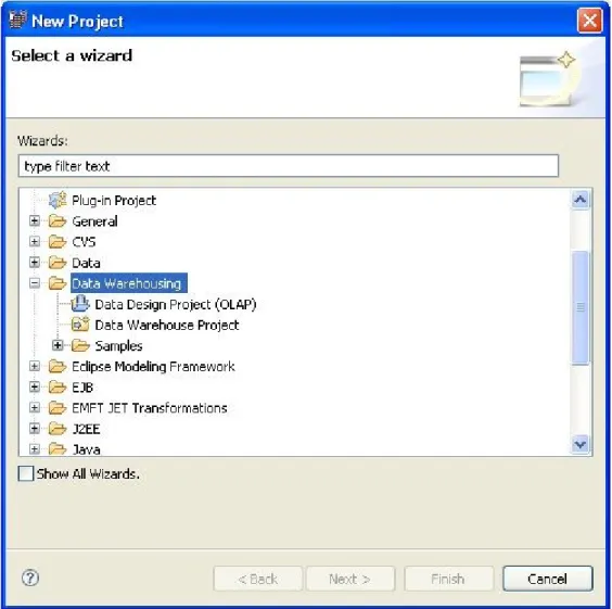
Creation of the data design project
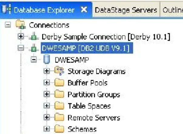
Reverse Engineering the existing database
It is possible to have a graphical representation of both schemas from the Data Diagrams folder in the project explorer. The data model must be opened and expanded to have diagrams in the data diagram directory).
Working on the physical data model
Defining the problems
Adding Primary keys
Adding Associations – Foreign keys
So this can only be used if the names of the columns in the fact table and in the dimensional table are similar.
Validation of the model
In this tutorial, the fact table and one dimensional table will be loaded.(When we can do it for one dimensional table, we can do it for the other. The goal is to understand the mechanism). SUBDIV.OU_IP_ID, -- ID of the subdivision of the store -> In the data flow replaced by the name (JOIN WITH IP). The input port of the operator will be linked to the data set of the Organizational Unit.
IN2_09.EFF_DT The date is stored in the table ITM_TXN and. different representations of this date in the MSR_PRD table. In a data warehousing application, the data flow consists of the base layer of the application.
Propagation of the modification on the database
The Comparison process
The comparison is useful because it provides an overview of the changes that have been made. This report shows that there are no foreign and primary keys in the DWESAMP:DWESAMP.MARTS schema, but they are present in the data model. We can discard the changes to the data model (it will change the schema to be the same as in the database), or propagate the changes to the database.
Our goal is to propagate changes to the database, so the run button is pressed from right to left. In the report, the edits are now propagated, but they are not yet in the database.
The DDL script
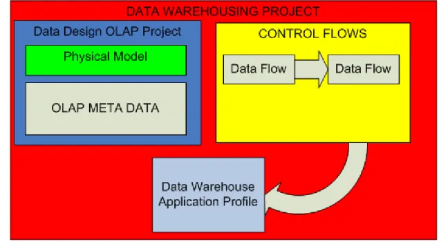
The data warehouse project
Introduction
What provides this project?
Definition of a data flow in Design Studio
Definition of some data flow operators
- File Import operator
- File Export operator
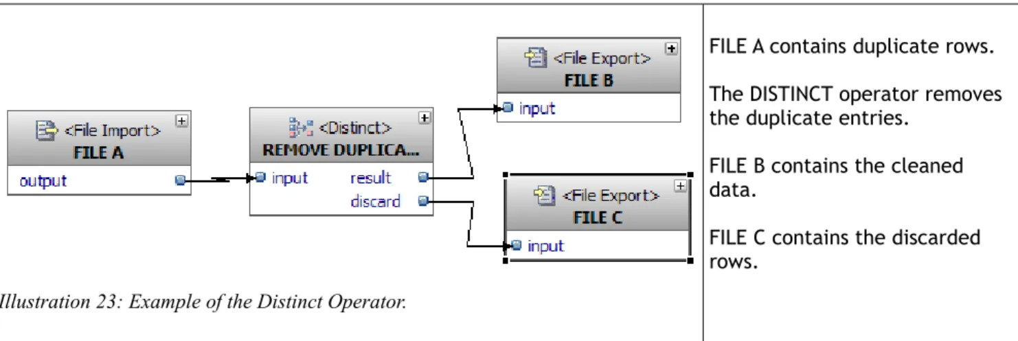
- Distinct operator
- Union operator
- Table Join operator
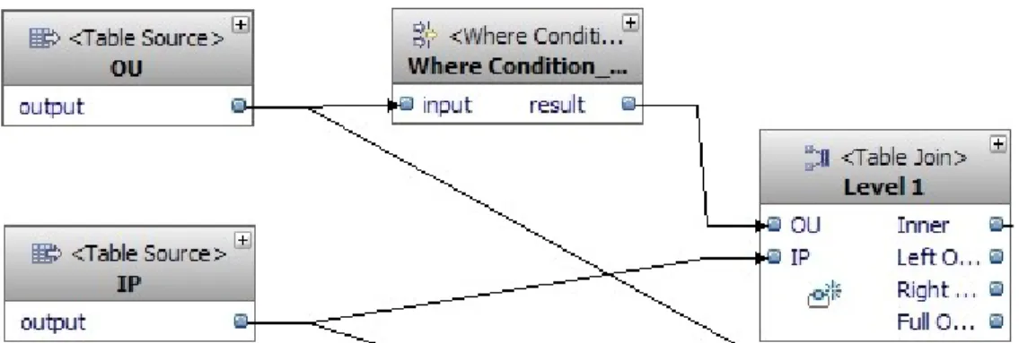
- Select List operator and Where Condition operator
- Key Lookup operator
- Easy to understand operators
The Table Join operator also has a Select List option that allows column selection in the design part of the query. This operation in SQL is called SELECTION and should not be confused with the projection that uses SELECT in the query. In illustration 26, the file import operator feeds the Item Transaction table with the day's sales.
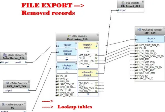
The key lookup operator will check if the sold product exists in the PRODUCTS table. On the other hand, the destination table operator feeds a table of data into the input port.
Data flows in the JK Superstore
Populating the Item Transaction table
Origin of the data and start point of the flow
Cleaning the data
For each lookup port of the key lookup operator, the matching condition must be constructed so that the operator knows hex column to be compared. This tool allows you to create SQL state with the mouse by clicking on inputs, keywords, operations and functions. The data station operator is an intermediate stage, where data can be entered into a step table to check the flow content at any moment in the data flow.
By right-clicking on the data station, we can retrieve data about the data flow. The contents of the displacement table are cleared before each run of the data flow.
Populating a dimensional table of the marts schema
- Origin of the data
- Explanation of the problem
- Resolving it within an SQL query
- Designing the first level
- Designing the other levels
- Overview of the data flow
SELECT STORE.OU_IP_ID, -- Id for the store STORE.OU_CODE, -- Code for the store. STORE.ORG_IP_ID, -- Id of the organization the store has for STORE.PRN_OU_IP_ID, -- Id of the subdivision of the store. REGION.OU_IP_ID, -- Id for the store's region --> same as above DISTRICT.OU_IP_ID -- Id for the store's district --> same as above FROM DWH.OU SUBDIV,DWH.OU REGION,DWH. OU DISTRICT,DWH.OU STORE,DWH.CL CUSTOMERS WHERE SUBDIV.PRN_OU_IP_ID IS NULL --> LEVEL 1 Subdivision is rows without parent AND SUBDIV.OU_IP_ID = REGION.PRN_OU_IP_ID --> LEVEL 2 which has LEVEL .
The first level of the hierarchy is the organization level and is characterized by a null value in the parent column. A Where condition operator holds this hierarchy level with a condition "INPUT_03.PRN_OU_IP_ID IS NULL".
Populating a fact table
Origin and details of the data
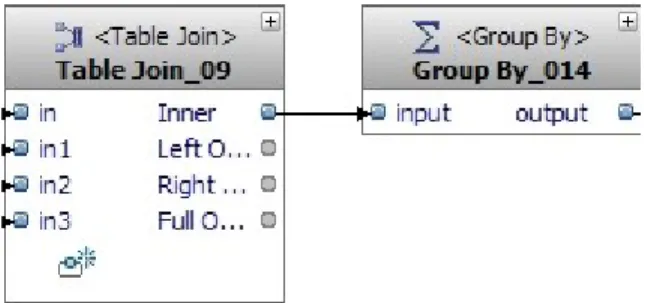
IN1_09.MKT_BSKT_TXN_ID Join the market basket transaction using the Item Transactions table. IN1_09.PD_ID = IN3_09.PD_ID Connect a transaction item to the product table to get information about the products (expected sales price,..). In addition to the previous operators for joining tables, we start by aggregating the data by using a "Group By" operator and defining the calculation of the various analyzable values in the operator's pick list properties view.
The Group By column is defined in the Group By tab of the property view.
Using the Key lookup operator
In the opposite, there will be many endpoints that represent the end of the process. On the other hand, errors can also be traced from the Websphere application server log files. At this part of the project, the data warehouse is completed and automatically updated.
Days after days the size of the warehouse increases and the data mining can be a good way for the analyst to find knowledge in the data. We are going to use it to interpret the result of the data mining on the JK-Superstore.
Overview of the flow
Definition of a control flow in Design Studio
A control flow is a graphical representation of the execution order of data flows that must follow a specific sequence. The second level is the control flow and is designed as the data flow in the data warehousing project. To create a control flow in the data warehouse project, we right click on the control flow directory and click on new Control Flow.
A control flow can be in a different project than that of the data flow, but to have a good project management and to make it easy to create the data warehousing application, it is better to use the same project.
Rules and operators from control flows
Rules
Outputs
Definition of available control flow operators
- Start operator
- End operator
- Fail operator
- Data Flow operator
- File Wait operator
- Stored Procedure operator
- Email operator
And calling these data flows in a control flow is the second level in developing a data storage application. The output of the operator is a little different from the others, but it is quite clear. The number of times the loop should be performed is defined in the operator properties view and can be set in three different ways.
If a new store appears, the store is added to the file and the data warehousing application will also extract the data from the new store (No need to reinstall the application, only the configuration file changes). This operator is used to send a mail that can alert the administrator about the use of branch in a control flow.
Using the control flow to feed the MARTS schema
Process understanding
Designing the data flows
Introduction
Deployment preparation
Working with DWE Administrating console
Prerequisites before deploying the application
Deploying the application
JK Superstore builds the Data warehouse
What is the data mining?
Why using data mining?
The
The goal of the data mining will be to find clusters, to regroup victims into different segments depending on certain characteristics. The Java code is available in the appendices, but here is some explanation about the Java Bean. Data mining is a fantastic tool, but it requires a very good understanding of a company's needs before it can be integrated into their system.
Creating the model that calls the Easy Mining For BASIC data mining sqlStmt = new StringBuffer();.
Association rules
Easy mining procedures
- Introduction to Easy Mining
- FindRules
- ClusterTable
- The others functions
A model is stored in the database if the stored procedure created the view and added the model to the model list table. For example, it could be used to share mining results between heterogeneous RDBMS (Oracle and I.B.M. DB2). Syntax: ClusteTable procudure IDMMX.ClusterTable(
Association rules on the Market Basket of JK Superstore
- Introduction
- Cleaning the data and Creating a model
- The visualizer
- Interpreting the result of the data mining
Our goal is to find relationships between products and more precisely according to the product category, which will be realized through operator associations. We will also need the products table to do the product name mapping. This model will be loaded in the visualizer to get the result, but it will also be used with the rule extractor to populate the view with the rules.
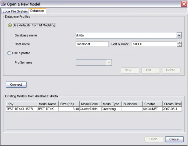
We come directly in front of the panel that makes it possible to connect to a database, get the list of models and open a model. When people buy items from the "Hair Care" category and items from the Miscellaneous (which is a subcategory of Health and beauty), people also buy items from the Personal Hygiene in 90% of the cases.
Clustering on the titanic data set
- Introduction
- The origin of the data
- How to create a model without mining flow
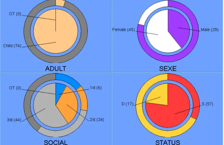
- Interpretation of the results
- The results with the geometric algorithm
SqlStmt currently contains: creating a time view, calling the data mining process, and creating a new view containing the data mining results. At the end of my training, I had the opportunity to present my work. The exercises presented at the ARISTOTEL University were proof of the success of the project.
I have worked for a fictional company, but in the future I hope to continue working in this field of data mining and KDD. On the other hand, an Erasmus project is also the best way to improve my English, learn more about foreign culture and also to get out of the 'family cocoon'.
The Java bean code to create the data mining model of titanic data set