66 Figure 83 Model accuracy and model loss (binary cross entropy) for excitation for the MLP-BP algorithm along with PSD and standard deviation for feature extraction in UC2 (male dataset). 71 Figure 101 Model accuracy and model loss (binary cross entropy) for Liking use for the MLP-BP algorithm along with STFT and standard deviation for feature extraction in UC2 (male dataset). 72 Figure 106 Model accuracy and model loss (binary cross entropy) for Valence for the MLP-BP algorithm along with STFT and Approximate Entropy for feature extraction in UC2 (male dataset).
72 Figure 108 Model accuracy and model loss (binary cross entropy) for dominance for the MLP-BP algorithm along with STFT and approximate entropy for feature extraction in UC2 (male dataset). 73 Figure 109 Model accuracy and model loss (binary cross entropy) for use for the MLP-BP algorithm along with STFT and approximate entropy for feature extraction in UC2 (male dataset). 75 Figure 117 Model accuracy and model loss (binary cross-entropy) for using liking for the MLP-BP algorithm along with DWT and standard deviation for feature extraction in UC2 (female dataset).
77 Figure 125 Model accuracy and model loss (binary cross entropy) for Like use for the MLP-BP algorithm along with DWT and Approximate Entropy for feature extraction in UC2 (female dataset). 79 Figure 133 Model accuracy and model loss (binary cross entropy) for Liking use for the MLP-BP algorithm along with PSD and standard deviation for feature extraction in UC2 (female dataset). 81 Figure 141 Model accuracy and model loss (binary cross entropy) for Like use for the MLP-BP algorithm along with PSD and Approximate Entropy for feature extraction in UC2 (female dataset).
82 Figure 146 Model Accuracy and Model Loss (binary cross entropy) for Valence for the MLP-BP algorithm along with STFT and Standard Deviation for feature extraction in UC2 (female dataset).
INTRODUCTION
High Level Architecture
The current thesis will make use of the DEAP database which will be presented in the following chapters. This component will be responsible for searching for the best features that accurately describe the dataset and are intended to be informative and non-redundant. By using data augmentation on the output of the feature extraction methods, we can significantly increase the diversity of data without actually collecting new one.
The feature vectors produced by the feature extraction and data augmentation stages contain many random variables and carry a lot of information. After identifying the appropriate feature vectors, it is time to implement and validate various classification methods to predict the class to which each of the feature vectors belongs. Emotion mapping is a process where the emotion-related labels predicted by the previous stage (classification algorithms) are mapped to the four basic and strong emotions as described earlier (happy, sad, angry, excited).
The output of the machine learning framework presented above is a music recommendation system, which is able to suggest music and songs that fit the users' mood. The current thesis will make use of the LAST.FM database to retrieve the proposed music and songs.
VALIDATION METRICS
DISCOVERING KNOWLEDGE
Supervised Learning
METHODOLOGY
- Data Sources Identification
- DEAP Database
- Description of Dataset
- Description Of Use Cases
- Feature Extraction Methods
- Discrete Wavelet Transform (DWT)
- Short Time Fourier Transform (STFT)
- Power Spectral Density (PSD)
- Data Augmentation
- Dimensionality Reduction
- Principal component analysis (PCA)
- Classification Algorithms
- Support Vector Machines (SVM)
- k-Nearest neighbors (kNN)
- Naive Bayes (NB)
- Random Forest (RF)
- Multilayer Perceptron - Backpropagation (MLP-BP)
- Voting Classifier
- Emotion Mapping
- Music Recommendation System
The following figure is an overview of the feature extraction mechanism, illustrating all the components required to produce the feature vectors. Finally, to conclude in a 1x5 feature vector for each of the 32 EEG channels/sensors, we calculated the standard deviation and approximate entropy of the calculated coefficients (see Appendix I). STFT analysis is one of the techniques used to reveal the frequency content of the EEG signals at each point in time.
We applied the procedure described above to the 20% of the feature vectors included in the initial data set. More details on the exact number of key components used in our experiments will be given in Chapter 5. Training set: A large subset of input data used to fit the classification model (most times 80% of the original dataset).
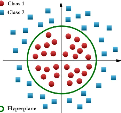
Test set: The rest of the data (20%) of the initial data set that will be used to evaluate our classification model is the test set. This distance from the decision surface (hyperplane) to the nearest data point determines the margin of the SVM classifier. Calculate the Euclidean distance between the new data point and the rest of the data points.
The figure above illustrates a high-level view of the Random Forest to better understand its logical steps. Training involves adjusting the weights and biases of each neuron (perceptron) in the model to minimize the error. The output of the network provides a prediction for each input fed to the neural network.
We fine-tuned all the ML algorithms presented in Chapter 4.5 by choosing the best values for their parameters to achieve the best performance for each of the 5 training models. To move forward, we combined the predictions from the 5 machine learning algorithms using the voice classifier. The pick was based on the genre, style and mood of the first music video.

EXPERIMENTAL RESULTS
Subject Independent Experimentation and Results
- Voting Algorithm Results and Recommendation List
Further on, Figures 21 - 28 show the accuracy and f1-score for all algorithms using the Discrete Wavelet Transform Feature Extraction Method together with Approximate Entropy (see section 4.2.1). Further on, Figures 37 - 44 show the accuracy and f1-score for all algorithms using the Power Spectral Density Feature Extraction Method together with Approximate Entropy (see section 4.2.3).

Gender Dependent Experimentation and Results
- Experimentation Results for the Male Dataset
- Experimentation Results for the Female Dataset
- Voting Algorithm Results and Recommendation List
Subject Dependent Experimentation and Results
- Voting Algorithm Results and Recommendation List
Next, Figures 164–167 present the accuracy and f1 estimate for all algorithms using the discrete wavelet transform feature extraction method together with approximate entropy (see Section 4.2.1). Next, Figures 168–171 present the accuracy and f1 estimate for all algorithms using the power spectral density feature extraction method along with the standard deviation (see Section 4.2.3). Next, Figures 176–179 present the precision and f1 estimate for all algorithms using the short-time Fourier transform feature extraction method along with the standard deviation (see Section 4.2.2).
Further on, Figures 180 - 183 show the accuracy and f1-score for all algorithms using the Short Time Fourier Transform Feature Extraction Method together with Approximate Entropy (see section 4.2.2).
CONCLUSIONS
There are some ideas that we would like to try in the future, such as other types of Deep Learning methods and more precisely recurrent neural networks (eg long short-term memory) that are best suited to time series problems. In statistics, the standard deviation is a measure of the amount of variation or spread of a set of values. A low standard deviation indicates that the values tend to be close to the mean of the set, while a high standard deviation indicates that the values are spread over a wider range.
The standard deviation of a random variable, statistical population, data set, or probability distribution is the square root of its variance. A useful property of the standard deviation is that, unlike the variance, it is expressed in the same units as the data. In statistics, an approximate entropy is a technique used to quantify the amount of regularity and unpredictability of fluctuations over time series data.