All the discussed methods of this thesis are closely related to the LT-related analysis of queuing systems and they are based on the latest NILT technology. The number of parameters to optimize increases with order in the "full" version of the optimization problem. The main difficulty of the transient analysis of PHMFMs is the proper description of the various borderline cases.
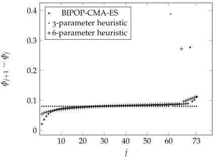
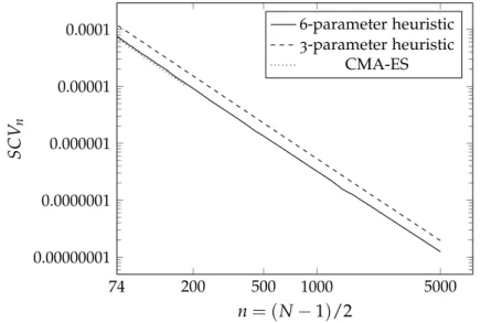
In general, the calculation of the moments µ0, µ1, µ2 based on (2.4), is not an easy task due to the computational complexity caused by the product of square cosine terms. The solution of the problem with the CMA-ES method [7] is fast, but it does not find the best optimum compared to the BIPOP-CMA-ES method [8], which is much slower. Figure 2.2 shows the location of theϕj parameters obtained by the full optimization method for n =74.
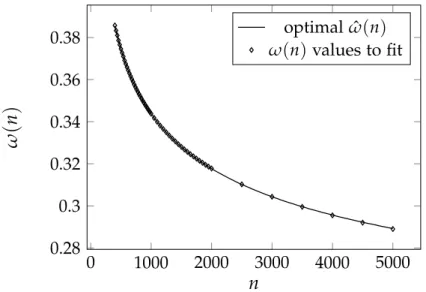
Figures 2.1 and 2.2 indicate that the equidistant location of parameters ϕj according to (2.7) is not flexible enough to achieve a similarly low SCV as obtained by the full optimization method. The intuitive meaning of the parameters in (2.11) is as follows: the meaning of p, w, ω and i is the same as in the 3-parameter optimization method, i.e.
The objective function of the heuristic method
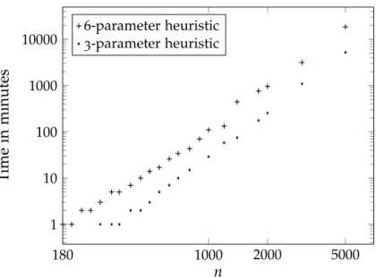
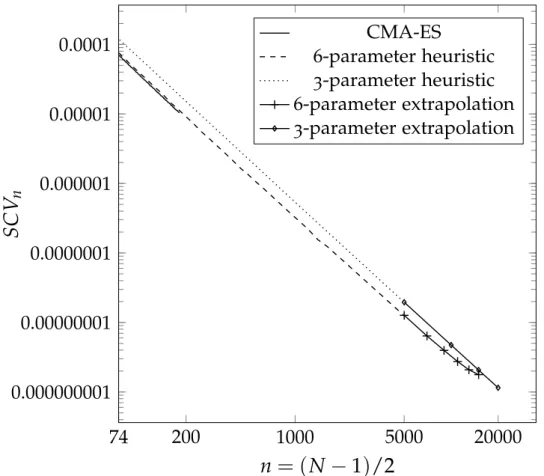
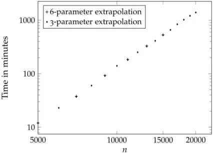
Figure 2.2: Location of ϕj parameters obtained by full optimization, 3-parameter optimization and proposed 6-parameter optimization for ordern=74. Figure 2.4: Running time of heuristic parameter optimization procedures for different orders in the log-log scale. SCV follows the same downward trend as the 3-parameter heuristic method up to the order of 5000.
Figure 2.7: Running time of the parameter approximation procedures for different orders in log-log scale. Most analysis results and application examples of QBD processes focus on the stationary behavior. Most of this chapter is devoted to the transformation domain description of the performance measures of interest.
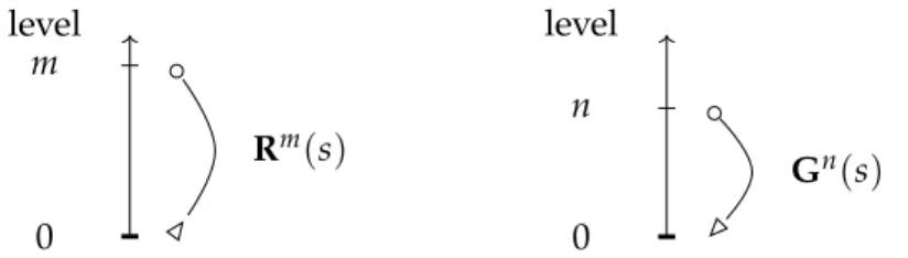
Most of the analysis is presented in section 3.5 and the summary of the proposed. At the thresholds, the behavior of the local transitions may deviate from the regular ones. In the following we will also make use of the G(s) and R(s) matrices of the level-inverted QBD (where the roles of the level-forward and level-back transitions are swapped), which are denoted by Gˆ(s) and Rˆ(s) and satisfy the quadratic equations.
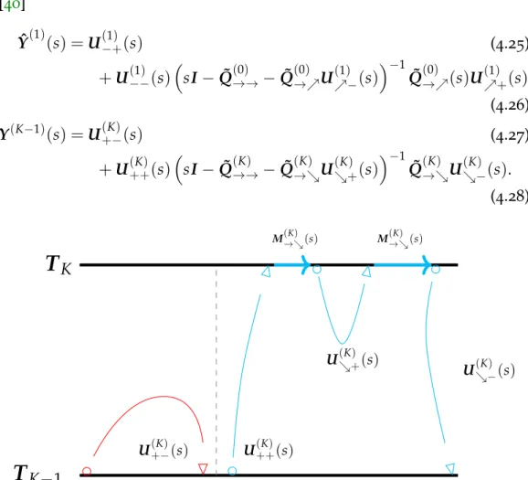
To express the LT of the transient distribution, we start by computing the first return probability matrices Y(s,n) and Yˆ(s,n), then the transient distribution at some specific levels (including the thresholds), and finally , from these auxiliary quantities we get the target quantity V(s,n,m). The first term of the left side describes the case that the process remains at level Tk for the entire period. The following theorem provides the LT of the transient distribution, given that the initial and the target levels are both thresholds.
The analysis of this case requires the following slight modifications of the above detailed procedure as follows. This chapter presents an analysis approach for LT description of the transient behavior of PHQBD processes. To keep the complexity of the analysis fairly simple, we adopt the terminology and the boundary behavior used in [41].
To order the states according to the sign of the fluid velocities, we introduce the permutation matrix Z with the following properties. The special cases when the initial liquid level is one of the limits are (see Figure 4.1).
To avoid undefined stochastic behaviour we impose the following natural requirements on these sets
For these records, we assume appropriate use of associative matrices for filtering and reordering. In Section 4.5, we illustrate the use of filtering and reordering matrices and their implementation. The following subsections describe the main steps of the proposed transient analysis approach in the order of their execution in the implemented algorithm.
Since the sign of the fluid velocity may be different at T0 and in the range (T0,T1), the dimensional validity of the expression causes problems in writing. Feasibility of matrix operations is always guaranteed by condition1, i.e. in this case S↗(0)⊂ S+(1). However, the feasibility of matrix operations is always guaranteed by condition1, i.e. in this case S↗(0) ⊂ S+(1).
The return measures for the residual bounds are also discussed in [40] using an explicit approach, which results in analytically complex expressions to evaluate. Using this approach hides the analytical complexity of the required measurements of the matrix inverse operation. Figures 4.3-4.5, visualize all the possible paths for the transition target to move a boundary down according to Eqs.
If S→(k) = ∅ for an inner boundary, then the third block row and column in the expressions above vanish. Based on the boundary crossing measures, B(k)(s) and Bˆ(k)(s), the return measures for the inner boundaries can be calculated as follows. Result 1. We start the LT domain description of the transient behavior with cases where the initial and final liquid levels are boundary values.
Similar blockwise equations apply to V(s,Tk,Tk). 4.48) The first term in V↗↗(s,Tk,Tk) represents the fact that from level Tk a unit impulse results in the fluid density at level Tk at t =0. With this model definition, we only need to modify the analysis of the last region compared to the finite buffer case. The rest of the section collects the elements of the analysis, which must be modified when the buffer is infinite.
For having a consistent model the following requirements need to be satisfied
Our implementation makes use of the index list-based matrix definition available in many programming environments (including Matlab and Mathematica). The memory complexity of the procedure is dominated by storing the O(K2) P(s,Tk,Tℓ) matrices, resulting in a memory complexity of O(K2|S◦|2). The stationary measures in this example (e.g., the probability of full buffer) are evaluated in [38], and some transient measures (e.g., the return time distribution of the inner bound) are given in [40].
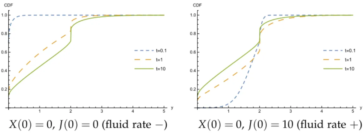
Figures 4.6 and 4.7 show the CDF of the liquid level distribution at time t, starting at state 0 (with negative liquid velocity) and state 10 (with positive liquid velocity) and from level 0 (empty buffer) and level 5 (full buffer). To overcome the difficulties, we introduce a hybrid algorithm, where the generator matrix of the modulation. The following section discusses the applicability of the EM method for MMFAPs and shows that the rate and variance parameters cannot be optimized.
Finally, Section 5.6 presents numerical experiments on the properties of the proposed method, and Section 5.7 concludes the chapter. In this work, we are interested in the stationary liquid arrival process and assume that the initial probability vector of the background CTMC is α=π. In our case, the hidden variables are related to the trajectory of the hidden Markov chain, specifically.
Based on these hidden variables, the logarithm of the likelihood is calculated in the next section. The maximization step of the EM method aims to find the optimal value of the model parameters based on the hidden variables. They are obtained from the partial derivatives of the log-likelihood as described in Appendix B.1.
In the expectation step of the EM method, the expected values of the hidden variables must be evaluated based on the samples. Appendix B.2 provides the analysis of those expectations, leading to E(Fi(k)) =riE(Θ(ik)) and E. r2i, from which the zth iteration of the EM method updates the flow rate and variance parameters as. This result is in line with the results obtained for discrete arrival processes in [57] considering the special features of the fluid model.
This result is in line with the results obtained for discrete arrival processes in [57] considering the special features of the fluid model. That is, we
The implementation of the EM-based parameter estimation method contains some complex elements that influence the computational complexity and the accuracy of the calculations. For the first estimates of the rest of the parameters, we have much less support from the measured dataset. The main problem is that the random effects of the Markov chain on the background and the variance of the fluid velocities cannot be easily discerned.
Under this assumption, one can obtain information about the "speed" of the background Markov chain as illustrated in Figure 5.3 in Section 5.6.1. To calculate the expected value of Θ(ik), the integrals of the forward and backward probability vectors must be evaluated. We note that these expressions give an interpretation for the zth iteration of the EM method forqi,j.
In the second case, it samples the accumulated liquid until the next measurement and maintains the state of the Markov chain. Similarly, we evaluated the EM-based MMFAP approximation defined in (5.16) based on 1000 samples starting with Q0=. The evolution of the value of the logarithm of the probability and the transition rates of the Markov chain along the EM iterations are shown in Figure 5.5a and 5.5b, respectively.
The evolution of the probability value during the optimization is shown in Figure 5.8, and the final probability is obtained by. The analysis of PHQBDs considers new performance measures based on a linear combination of series of MGs in each buffer region, which are related through boundary equations. For this, I introduced a set of benchmarks based on matrix inversion instead of the direct analysis approach used for homogeneous MFMs.
The estimated parameters are those that maximize the log-likelihood of the sample series. Another recent application of the CME NILT method was the transient analysis of message propagation for Vehicle Ad-hoc Networks (VANETs) with Disconnected Roadside Units (RSUs) [66]. The recent application of PHMFM transient analysis has yielded the reliability of millimeter wave (mmWave) radio, which is a key building block in 5G cellular networks [84].
Rechargeable batteries are one of the most important resources in many areas of today's life, e.g. in electric vehicles (EVs). Analytical solution of the pollution transport equation with variable coefficients in river using the Laplace transform.” In: Water and Irrigation Management pp.683–698.