MNB Background Studies 3/2002

MNB Background Studies 3/2002

Gábor Pula and Ádám Reiff

C

-

H

?

September 2002

Online ISSN: 1587-9356

Gábor Pula, analyst, Economics Department, Conjunctural Assessment Division E-mail: [email protected]

Ádám Reiff, CEU Ph.D student E-mail: [email protected]

MNB Background Studies comprise economic analyses related to monetary decision- making at Magyar Nemzeti Bank. The aim of this series of studies is to increase the transparency of monetary policy. Thus, as well as technical issues of forecasting, selected background material on economic issues that crop up in the course of the decision-making process is also published. The studies are released only in electronic format.

The analyses reflect the authors views, and they do not necessarily reflect those of Magyar Nemzeti Bank.

Magyar Nemzeti Bank 8-9, Szabadság tér

Budapest, 1850 http://www.mnb.hu

Abstract

In this study we investigate the usefulness of business survey data in forecasting Hungarian manufacturing output growth in the short run. We analyse the individual questions of the business surveys, and use models with different flexibility (factor model, best fitting and recursively best fitting model) to estimate the relationship between the business survey indicators and manufacturing output growth. The models are evaluated according to their forecasting performance. We generally find that confidence indicators can be useful in forecasting manufacturing output in the short run. However, the forecasting ability is limited to a one-quarter horizon.

Consequently, indicators of business activity can only be used restrictively, mainly in the context of a ‘nowcast’ approach.

Table of Contents

Introduction*...5

The dataset ...6

Data stationarity and detrending...7

Analysing the relationship between manufacturing output and indicators of business activity...8

The model-building framework...12

Estimating the models ...15

Evaluation of forecasting results ...16

Summary and directions of further research ...18

References ...19

APPENDIX A ...21

APPENDIX B ...26

Introduction*

Last year, the level of domestic manufacturing output fell for the first time in many years. A decline in external demand was responsible for the interruption of the earlier upward trend, indicating that domestic economic developments were becoming more and more synchronised with global business cycles. Internationally, business surveys are used extensively to forecast business cycles as they are published quickly, ahead of official statistical releases. Although indicators of business activity enjoy increasing popularity among Hungarian economic analysts, we have relatively little experience in respect of the contents and usefulness of data.¹

The aim of this paper is to analyse information that can be derived from business surveys and to decide whether business sentiment indicators can be used to forecast manufacturing output in Hungary.² There is a wealth of information in international academic literature about the forecasting properties of sentiment indicators.

Experience has shown that business sentiment variables are suitable for forecasting industrial cycles in most countries. Santero-Westerlund (1996) conducted cross- correlation analyses on a group of OECD countries. Their results show that sentiment indicators are good predictors of both manufacturing output and fixed investments activity. According to the findings of Mourougane-Roma (2002), the sentiment index of the EU is suitable for forecasting GDP growth in the six largest member states of the EU. The results of Camba-Kapetanios-Smith-Weale (2000) provide evidence that models based on sentiment variables have a better predictive power in both the United Kingdom and the United States than alternative autoregressive models. However, these papers also demonstrated that sentiment indicators only aid forecasts over a relatively short horizon, i.e. over maximum three months.

According to a large portion of international experience, not only the short horizon is viewed as the biggest problem encountered in using sentiment indicators. Roberts- Simon (2001) maintain that responses to business surveys tend to be influenced by economic data released earlier, and so sentiment indicators do not convey any additional information relative to available ‘traditional’ statistical data. In their paper, the authors demonstrated that, after eliminating the effect of ‘traditional’ statistical data, the sentiment variables lose their predictive power. The subjective nature of responses to business surveys represents another problem. Due to the subjectivity inherent in responses, the relationship between sentiment indicators and economic variables measured by traditional statistics is much more volatile than that between purely economic variables. As a result, the forecasting properties of models employing sentiment indicators are highly sensitive to the number of observations (Camba-Kapetanios-Smith-Weale (2000)) and the detrending methods applied to time

* We are greatly indebted to Mihály András Kovács and Gábor Vadas for their useful comments, as well as to Ágnes Nagy (KOPINT) and Raymund Petz (GKI) for making the data available.

1 The paper by Tóth (2002) provides a comprehensive description of the statistical peculiarities of household and business surveys. Vadas (2001) summarises experience related to household sentiment indices. On the use of household sentiment indices in forecasting consumption expenditure, see the paper by Jakab-Vadas (2001).

2 Hereinafter, we call sentiment indicator or sentiment variable those economic variables, which we produce from the individual questions in business surveys. We refer to the officially released business activity indicators that are weighted from the questions, as composite indices.

series (Weale (1996)). The instability of this relationship requires flexible modelling techniques, for example, the Mourougane-Roma (2002) model estimation method based on time-varying parameters or the forecasting models constructed by Blake- Kapetanios-Weale (2000) applying the procedure of a recursive estimation techniques.

In Hungary various attempts to use sentiment indicators were already made in the mid-1990s – the common objective of the papers by Hoós-Muszély-Nilsson (1996) and Reiff-Sugár-Surányi (1999) was to develop a leading indicator of Hungarian industry. In the course of their examinations, both group of analysts found that Hungarian sentiment indicators can only be used restrictively for forecasting purposes. The limited length of the available time series also played a role in the authors arriving at this conclusion.

The paper by Ferenczi-Reiff (2000), whose objective was also to develop a leading indicator to forecast future turning points of the business cycles, was a direct blueprint for our study. According to its findings, although sentiment indicators can indeed be used for forecasting purposes, their application produces an improvement in the effectiveness of forecasts only over relatively short periods of maximum three months. On the other hand, in respect of data detrending a store of experience has been accumulated since the conclusion of their research project primarily, which we attempted to utilise throughout our analysis.

In the first part of our paper, we deal with the underlying data, their stationarity and the chosen detrending method. Afterwards, we analyse the relationship between manufacturing output and business surveys, with the help of statistical methods widely used in academic literature (cross-correlation, Granger causality test). We conducted our analysis both on the composite indices and at the level of individual questions of the surveys. At the same time, though, these examinations also represent a method of choosing the sentiment indicators that are suitable for forecasting purposes. We tested the predictive power of business survey data with three various models, using the ARIMA representation of manufacturing output as a reference model. Finally, we present our major conclusions drawn from the evaluation of the forecasting errors of the models, and outline the possible directions of further research.

The dataset

In the course of our analysis, we used the data derived from the business surveys conducted by GKI and KOPINT. There are two reasons for the examinations being confined to these two data sources. First, Tóth (2002), in his review of domestic business surveys came to the conclusion that currently only the data series of KOPINT and GKI have the sampling and representativity properties which make them suitable for performing further statistical examinations. Second, these are the two business surveys whose end results, namely business confidence indicators, enjoy the greatest popularity among domestic analysts.

Table 1 of Appendix B provides a detailed description of the questions pertaining to the business surveys. As the paper by Tóth (2002) includes detailed sampling and

statistical characteristics of the business survey data, at this point we only discuss the method used for data transformation.

We performed our analyses at quarterly frequency, thus we had to cumulate GKI's data released with a monthly frequency.³ We accomplished this task by averaging the monthly data. The basic data are derived as the balance of positive (high/increasing) and negative (low/decreasing) responses given to the questions. The balances were increased by 200. This means that our variables are allowed to move in an interval between (+100)–(+300).⁴ We seasonally adjusted the KOPINT's data. However, we skipped this treatment in the case of the GKI's data, as the time series are published seasonally adjusted by the institution.

The overwhelming majority of questions in business surveys are formulated in a way that the increase in the balance of responses indicates a pick-up in business activity.

Questions relating to the expected level of finished inventories and capacities relative to future orders are an exception to this rule.⁵ We inverted these variables (i.e.

deducted them from 400), thus assuming a co-movement (i.e. a positive correlation) between the time series for manufacturing output and each sentiment indicator involved in the analysis.

Our reference time series is the time series for manufacturing output, which we also calculated on a quarterly basis by aggregating monthly data. The data were seasonally adjusted.

Data stationarity and detrending

We performed the stationarity test of data using three various unit root tests (see Table 2). In the case of manufacturing output all three tests (ADF, PP, KPSS) show equally that the time series of the process contains a unit root. However, our results were not unambiguous in the case of the sentiment indicators. The majority of the variables did not prove to be stationary on the basis of tests that postulate the presence of a unit root as a null hypothesis (ADF, PP test). By contrast, according to the KPSS test,⁶ in which stationarity is postulated as a null hypothesis, the overwhelming majority of time series proved to be stationary.

3 Two arguments supported the choice of quarterly frequency. First, the survey by KOPINT is only published quarterly, and so we did not have to express the quarterly data on a monthly basis using a method that would be difficult to defend in economic terms. Second, forecasting on a quarterly basis is consistent with the requirements of the forecasting practice followed by the MNB.

4 We ‘inherited’ this transformation by taking over the database of Ferenczi and Reiff (2000). They produced the detrended data as the ratio of the seasonally adjusted time series to their HP trends, thus they had to eliminate the non-positive values. As adding the constant does not have any consequence from the perspective of our final results, we maintained this form of the variables.

5 A rise in the current level of inventories shows increasing difficulties encountered in selling. If the level of production capacities is high relative to future orders for output, then neither sales nor fixed investment activity is expected to rise.

6 For a detailed description of the Kwiatkowski-Phillips-Schmidt-Shin (KPSS) test, see Kwiatkowski- Phillips-Schmidt-Shin (1992).

Theoretical considerations would underpin the stationarity of sentiment indicators, as these time series are only allowed to move within the confines of an interval.^TP7PT However, there are examples available in international literature of test results questioning the theoretical considerations. Examining a sample about four times longer than ours, Mourougane-Roma (2002) found that sentiment indicators contain a unit root. Adopting their practice, we decided to conduct the same analysis on both the level variables and their detrended time series in cases where the existence of stationarity was not obviously reinforced on the basis of the tests. As our main objective was to forecast for the short term, we decided the issue of using the level versus the de-trended data on the basis of their forecasting abilities.

Choosing the method used for detrending is a central issue from the perspective of further analysis. The most major experience of the period since the conclusion of the paper by Ferenczi-Reiff (2000) has been that the detrending technique they used (Hodrick-Prescott filter) greatly contributed to the increase in the out-of-sample forecasting errors of their models. For more details, see Appendix A.

In the light of experience discussed above, we decided to use the first-order difference (FOD) filter in our paper. This approach is supported by a number of arguments. First, in contrast with the Hodrick-Prescott (HP) filter, the FOD filter does not amplify the business cycle frequencies we intend to analyse, and so it certainly does not contribute to demonstrating irrelevant relationships. Second, using the FOD filter, it is not necessary to forecast a separate trend component and this, under our expectations, may improve significantly the accuracy of our forecasts.^TP8PT

Analysing the relationship between manufacturing output and indicators of business activity

GKI's industrial confidence index and KOPINT's manufacturing confidence index are the two indicators monitored most widely by domestic economic analysts. Comparing the confidence indicators of the two research institutes with the time series of the quarterly change of manufacturing output, we may assume that these indicators tend to lag rather than lead changes in manufacturing output. This hypothesis will be analysed in greater detail throughout the various stages of the analysis.

TP

7

PT The shortness of the time series reduces the power of the otherwise unrobust unit root tests. This may argue in favour of the stationarity of sentiment indicators.

TP

8

PT For detailed description of the FOD and HP filter deternding techniques, see the articles by Canova (1998), Harvey-Jaeger (1993) and Nelson-Plosser (1982). For a comparison of the various detrending techniques applied to domestic data, see the paper by Jakab-Kovács-Lőrinc (2000).

Chart 1 Manufacturing output and business confidence indicators

-2 -1 0 1 2 3 4 5 6 7 8

1q95 3q95 1q96 3q96 1q97 3q97 1q98 3q98 1q99 3q99 1q00 3q00 1q01 3q01

quarter-on-quarter, percent

-15 -10 -5 0 5 10 15 20 25

balance

Manufacturing output

GKI industrial confidence indicator (right scale)

KOPINT manufacturing confidence indicator (right scale)

There is domestic experience in respect of the weak forecasting ability of composite indices. According to the calculations by Vadas (2001), GKI's consumer confidence index lags behind changes in the time series of consumption. The author concluded that, in this case, it is useful to perform an examination of the business surveys at the more disaggregated level: at the level of the individual questions. The reason for this is that, in compiling composite indices research institutes adopt the Eurostat's practice which may lead to false results if applied to Hungarian data.⁹ Analysing at disaggregated level we may find questions that have more favourable forecasting abilities than those in the official composite indices. By weighting these questions together we can produce a more useful composite index for the purposes of forecasting. Based on the recommendations by Ferenczi-Reiff (2000), Tóth (2000) and Vadas (2001), we also conducted our analyses on the question-level data.

Following Vadas (2001) we used three methods in the case of both the levels and the detrended (first-differenced) series to analyse the relationship between manufacturing output and business survey data (confidence indicators). As a first step, we used the indicators of cross-correlation and correlation asymmetry. Then, we quantified the additional explanatory power of business activity indicators. Finally, we tested the Granger causality existing between the reference time series and the business activity indicators. We conducted the analysis on the entire sample, i.e. the period 1995 Q1–

2001 Q4. In each case, the reference time series was the first-differenced time series for manufacturing output.

The purpose of the cross-correlation analysis is to define a number of lags at which co-movements in the reference time series and the confidence indicator examined are the strongest. Provided that this number of lags is negative, the confidence indicator

9 Both GKI's and KOPINT's sentiment indices are assembled by weighting together three questions of the business survey. These are the production perspectives, the assessment of existing orders and the level of finished inventories.

leads the time series for manufacturing output, and so it can be used directly for forecasting purposes. Conversely, if the lag is positive, then the business activity indicator ‘only’ lags variations in output and, consequently, it cannot be used for forecasting purposes.

Typically, correlation is not symmetrical around the number of lags resulting in the strongest co-movement. It may happen, for example, that the strongest co-movement materialises with a 0. lag, that is, the sentiment indicator is coincident with industrial output; however, correlations pertaining to the negative lag, showing a lead, are larger than those pertaining to the positive lag. This effect is measured by the indicator of correlation asymmetry, whose negative value expresses the lead of the examined time series vis-à-vis the reference data, while its positive value shows a lag.

In performing the cross-correlation analysis, we found that negative correlation values emerged even at a very low number of lags. This appears to be in contradiction with our starting hypothesis, according to which sentiment indicators are positively correlated with manufacturing output. That result shows the fragility of the relationship analysed; and it is also a warning that one must be very circumspect in the further steps of the examination. The reason is that there is a high likelihood of the effects of negative coefficients appearing in our results, in addition to the theoretically sustainable positive relationships. In order to address the above anomaly, we excluded lags having negative coefficients from the further analysis. Tables 3 and 4 of Appendix B show the results of the cross-correlation analysis applied to the levels and the de-trended time series. The second column of the tables contains the number of lags ensuring the strongest co-movement, the next column showing the value of the correlation asymmetry. The last column of the table contains the significance of the correlation value.

In the second step, we analysed whether the sentiment indicators provided any additional information about manufacturing output which was not present in past developments (autoregressivity) of the production process itself. Expressed in other words, this issue is about whether the accuracy of forecasts of output can be improved by taking into account developments in sentiment indicators, in addition to past information directly relevant to output. In order to answer the question, we involved the coincident and lagging values of the various sentiment indicators in the equation containing the best ARIMA representation of manufacturing output, and analysed the extent to which the explanatory power of the equation improved. We eliminated the lags having negative coefficients from the equations. Tables 5 and 6 contain both the adjusted increment R² and the combined significance of the variables involved. The table clearly shows that a number of variables, proving significantly leading during the cross-correlation analysis, do not improve the explanatory power of the ARIMA models and so, presumably, they do not enhance the accuracy of the forecasts either.

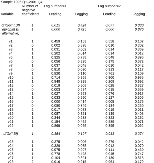
For the purposes of analysing the predictive power of sentiment indicators, we also tested the Granger causality between manufacturing output and sentiment indicators.

This test can be performed in two ways. First, one can examine the extent to which the leads of a given sentiment indicator explain variations in output (to what extent the indicator can be viewed as the leading indicator of output). Second, one can also test the extent to which the leads of output explain variations in the sentiment indicator (to what extent the indicator is lagging output). Obviously, the more likely a

sentiment indicator proves to be a leading index and the less likely it proves to be a lagging index, the more applicable it is for forecasting purposes. The results of the Granger test are included in Tables 7 and 8. We also indicated the number of negative coefficients of the Granger test equation in the first column of the table. The higher the number of negative coefficients in the equation, the less we view the results of the Granger test as substantial in economic terms.

Summarising the results of the three methods discussed above, the following observations can be made about the relationship between manufacturing output and sentiment indicators:

We obtained five variables during the examination of the level time series of sentiment indicators which, based on the tests, show a close co-movement with manufacturing output:

• position of the firm over the next six months (q12)

• production of the firm over in the next six months (q13)

• volume of the firm's domestic sales over the next six months (q14)

• volume of the firm's sales to EU over the next 6 months (q16)

• volume of the firm's total sales over the next six months (q17)

These sentiment indicators have two categories from the perspective of maximum correlation. They are either coincident, with positive correlation asymmetry, or lag one quarter, but have a negative asymmetry value. Both cases mean that our indicators lag one to two months. It is a positive property of the chosen indicators that, in addition to the autoregressivity of output, they contain additional information about developments in output. However, in the case of these time series, we could not demonstrate a significant leading relationship using the Granger causality test (except in the case of q13). This suggests that these variables can only be used restrictively for forecasting purposes – they are suitable for nowcasting.^TP10PT

The differentiated time series show a more favourable picture than the above. Here, we found six variables that could be useful for longer-term forecasting, in contrast with the level variables:

• firm's production in the past quarter (v2)

• current level of EU orders (v6)

• position of the firm over the next six months (v12)

• production of the firm over the next six months (v13)

• volume of the firm's domestic sales over the next six months (v14)

• volume of the firm's sales to EU over the next six months (v16)

Based on the Granger test, these indicators lead the time series for manufacturing output by one quarter, in addition to the high cross-correlation values and additional

TP

10

PT The essence of nowcasting is that we provide an estimate of the actual data with a sentiment indicator referring to the same quarter. Actually, this estimate means a one-month forecast, as the business surveys provide information about the given quarter one month ahead of the official statistics.

The results of both the GKI and the KOPINT surveys are made available within 15 days following the reference period. By contrast, the CSO only releases detailed data on manufacturing output some 45 days after the reference quarter.

explanatory power, so, one can also use them to forecast output on the horizon of one quarter.

In the case of the level of composite indices, the results clearly reinforce our initial assumption that, in their current form, business confidence indicators as published by the research institutes are not suitable for forecasting future variations in manufacturing output. Although they co-move with output, they follow it with a lag and, moreover, they do not include any additional information relative to past developments. The most major reason for this is that, except in the case of the outlook for output, the variables in the composite indices themselves did not prove to be good predictors either.

By contrast, the results of the test showed that changes in the KOPINT's composite index (the differentiated time series) can be useful to forecast short-term variations in manufacturing activity. With differentiation, the lead of the composite index and its explanatory power both increased robustly. However, there remained variables within the components of the composite index, which did not prove to be good predictors.

Therefore, we also produced an alternative index by weighting together the variables, which can be viewed as good predictors.

Although, based on the test statistics, the alternative index was found to possess excellent forecasting properties, there appear to be obstacles to its wider practical use.

The reason for this is that, to produce the alternative index, question-level data are required as well, which cannot be found in the official publications. Consequently, as a compromise, monitoring the changes in the official composite index can be a solution in practical applications.

In the case of the GKI composite index, neither its variations nor the questions in the GKI poll themselves proved to be good predictors. Consequently, we cannot make an alternative proposal for practical use of the GKI composite index.

The model-building framework

The tests performed in the previous chapter demonstrated that the questions in business surveys contain information that helps to forecast the changes in manufacturing activity. In the following, we seek to answer the question of which model-building procedure should be chosen in order to make our forecast the most accurate.

In order to answer the question, we employ three different model-building procedures using both the level and the differentiated time series. These are the principal component-based model, and the ‘best fit’ and ‘recursively best fit’ models. We chose one quarter as the forecast horizon; and we defined the forecasting accuracy of the models with the help of the root mean squared error of their out-of-sample forecasts.

Each of the models constructed contains a constant, the value of the dependent variable lagged by one quarter, as well as the coincident and lagging values of the sentiment indicators. However, the selection of the sentiment indicators built in the models, follow different mechanisms in the case of the three model-building techniques.

The principal component-based model contains a principal component as an explanatory variable, in addition to the constant and the value of manufacturing output lagged by one quarter. The principal component was generated from the variables, which we chose with the help of tests described in the previous chapter.

Accordingly, the principal component basically corresponds to the alternative indicator we created, with the difference that the variables are composed by using the principal component weights. However, we made this choice on a narrower sample for the period 1995 Q1–1999 Q4, in order to be able to quantify the errors of out-of- sample forecasts. The change in the sample slightly alters the range of the chosen sentiment indicators. In the case of the level time series, only the question regarding to total sales was kept of the questions asked about the sales outlook, while future developments in numbers employed became a good explanatory variable. In the case of the differentiated data the question of outlook for EU orders was replaced by the outlook for exports to the CIS.¹¹

Of the model specifications we use, the principal component-based model is seen as the least flexible one. We define the concept of flexibility on the basis of three factors, consistent with the paper by Blake-Kapetanios-Weale (2000). We consider a model- building technique ‘absolutely’ flexible if

1 it allows sentiment indicators to have different numbers of lags in the model, 2 it uses the various groups of sentiment indicators as explanatory variables over

the different sample periods, and

3 it generates models on the different forecast horizons which are based on the different groups of sentiment indicators.

Given that sentiment indicators reflect subjective judgements and expectations, they are in a less robust relationship with other economic variables, in comparison with statistics taken in the traditional sense. Conceivably, some of the questions may contain relevant information from the perspective of manufacturing output in the upward phase of the business cycle and some others during a recession. Our examinations showed that the explanatory power of the variables may change drastically at the various lengths of the sample period – for example, in the first half of 1999, a large part of the indicators that fitted well in the previous period lost their explanatory power. In a similar vein, it is also conceivable that different groups of the sentiment indicators possess strong explanatory power on the various forecast horizons. Accordingly, the property of flexibility means the extensive use of all available information.

We deem it very important to stress, however, that, with the enhancement of the flexibility of the model, we have to face two significant problems. First, using flexible models increases the probability that a noise at the end of the sample would largely distort our forecast. Second, with the possibility that the range of variables in the forecast may change from quarter to quarter, the evaluation of the forecasting errors and the comparison of the forecasts performed at various points of time become very complicated tasks. We will discuss these difficulties in more detail when evaluating the results.

11 In the case of level data, our main component explains 84% of the combined variance of the four chosen variables (q12, q13, q17, q19). In the case of the detrended data (v2, v12, v13, v14, v15, v16), this ratio is only 55%.

The principal component-based model does not satisfy either of the flexibility criteria.

This suggests that the model does not make use of the full range of available information. Taking the paper by the Blake-Kapetanios-Weale (2000), we tested two different model-building techniques, in order to enhance the effectiveness of our forecasts. The best fitting model satisfies the first and last criterion of flexibility, while the recursively best fitting model satisfies all three criteria, and so it can be viewed as absolutely flexible.

In the best fitting model, each one of the lags of the sentiment indicators is treated as a separate variable. In the first step of the procedure, we ranked these variables depending on the degree of their ability to explain fluctuations in manufacturing output. (Naturally, we excluded variables with negative coefficients from the analysis.) In the second step, we generated all possible combinations of the five best fitting indicators, which we used to build 31 models.^TP12PT As our purpose was to employ the simplest possible models, that is, which contain the least of explanatory variables, we ranked the models on the basis of the Akaike information criterion (AIC), and chose the one having the lowest AIC value as the best fitting model. We carried out this model-building procedure on both forecasting horizons (nowcast and a forecast for one quarter).

The best fitting model can be very sensitive to the choice of length of the estimating period. This stems from the possibility that, while a model fits well in the middle range of a sample, it fits less well at the end, and in this case it cannot be viewed as a best fitting model. In order to eliminate this deficiency, we can use a model-building technique, which re-iterates the choosing and estimating steps of the best fitting model described above in each period. This is the model of the recursively best fit, which may not only mean different specifications on the various forecast horizons, but it may also result in the replacement of the explanatory variables in each case when our sample is expanded with a new data point.

The table below summarises the systematisation of our models.

Model Sentiment indicators with different numbers

of lag

Different sentiment indicators on different

estimating sample periods

Different sentiment indicators on different

forecasting horizons Principal component-

based model No No No

Best fitting model Yes No Yes

Recursively best fitting

model Yes Yes Yes

TP

12

PT If the number of the chosen variables is denoted with q, then number of all possible variations that can be generated from them is 2q−1. The above description, referred to as data-snooping in the literature, is a particularly widely used tool in analysing financial markets. As the procedure does not employ restrictive assumptions in respect of the selection of explanatory variables, it often produces relationships known as spurious regressions, when applied. A number of methods have been devised to handle this problem. For more details on this and the data-snooping procedure, see the paper by Timmerman-Sullivan-White (1998).

Estimating the models

We estimated our models on the sample period between 1995 Q1–1999 Q4.

Originally, we made an attempt to specify models forecasting for two quarters, but we did not find a sentiment variable on this forecast horizon which would have proved to be significant. Accordingly, our models only cover two forecast horizons (nowcast and a forecast for one quarter). The estimating procedure was the same in the case of all three models; we then estimated the models in a system of equations, in the form as shown below:

t j

i t j

t

t d feldterm konj u

feldterm

d^{log( )}=^α +^{β1* log( −1)}+

∑

1

1 2

1 1

1) * log( ) *

log(^feldtermt₊ = + ^{d feldterm∧ t} +

∑

d γ ϕ ϕ ε (2)

where dlog(feldterm^∧ _t) is the forecast of manufacturing output in equation (1) chosen for nowcasting. (In this set of equations, konj^P1PB_t-i^B and konj^P2PB_t-i^B denote the groups of indicators involved in the equations, where the i number of lags can change between 0 and 2. Indices j and m denote the numbers of sentiment indicators included in the equations.)

Estimating in a system of equations serves the purpose of enabling ourselves to take account of the errors in the nowcasting equation in estimating the one-quarter forecasting equation, thereby enhancing the accuracy of the fit of the equations. As the forecast of equation (1) is included in equation (2), the residuals of the two equations will be correlated.^TP13PT Accordingly, we performed the estimation using the seemingly unrelated regression (SUR) method.^TP14PT

In arranging the order of the models, we used the AIC indicator of the systems of equations.^TP15PT

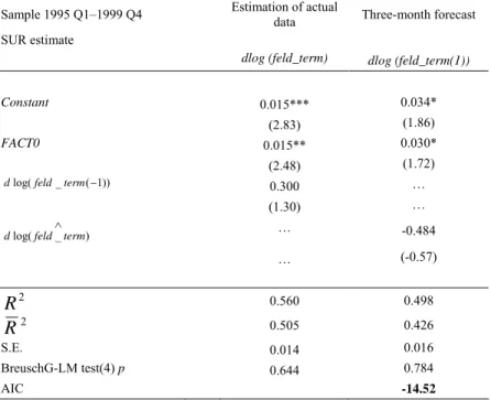
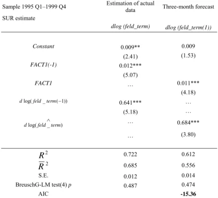
Tables 9 to 13 contain the results of the estimates. Our models possess a high R² and robust test statistics; and their fit is much better than that of the ARIMA model chosen as the basis of comparison.^TP16PT Differentiated data explain the manufacturing output better in the cases of both the principal component-based and the best fit models than the level time series. This discrepancy is particularly significant on the one-quarter forecast horizon. Of all the models, the principal component-based model, which contains the differentiated data possesses the lowest AIC indicator. Accordingly, this is the specification that describes past developments in manufacturing output the most

TP

13

PT The results of the formal likelihood test also appear to have reinforced the correlation of the differential variables of the equations.

TP

14

PT In contrast with the ordinary least squares (OLS) method, the SUR estimation method does not require that the residuals of the various equations to be homoscedastic and uncorrelated by pairs. The estimation procedure is based on the generalised least squares (GLS) method, where the variance- covariance matrices of the equation residuals can be derived with the OLS estimation of the equations.

TP

15

PT We calculate the AIC indicator of the systems of equations from the loglikelihood function of the system of equations (see note on Tables 9–11).

TP

16

PT The ARIMA representation chosen as the basis of comparison is actually an AR(1) model which we estimated on the basis of the procedure presented above.

accurately. However, as our purpose is to forecast for the short term, we rank the various model specifications on the basis of their forecasting abilities instead of the accuracy of fit. We made out-of-sample forecasts in order to perform this task.

Evaluation of forecasting results

We have tested the forecasting ability of the models over the 2000 Q1 to 2001 Q4 time horizon. Table 14 shows the root mean squared errors (RMSE) of the model forecasts. The table enables the following main inferences to be drawn:¹⁷

1 Consistent with our earlier findings, the fact that each model has a smaller forecasting error than the ARIMA specification proves that confidence indices convey additional information that can be used over the short term to improve the accuracy of forecasts relating to manufacturing output.

2 Having not found any one model specification in which the confidence indices have significant explanatory power after six-month lags, we concluded that the information provided by the business surveys facilitates forecasting over a maximum horizon of three months.

3 Of the models using either level or differentiated data, the latter exhibited the smallest forecasting error in most specifications. That is, using the differentiated data of the confidence indices makes for more efficient forecasting than using level series. The increase in efficiency is especially remarkable on the one-quarter forecast horizon.

4 On both forecast horizons, the recursively best fitting model, which uses differentiated data produces the slightest forecasting error. This good performance of the recursive model proves that the procedure’s sensitivity to ‘noise’ did not increase the forecasting error significantly. The principal component-based model that uses differentiated data also exhibits excellent forecasting properties. The principal component can also be viewed as an alternative corporate confidence index.

5 The poor performance of the best fitting model is due to the instability of the relationship defined by the sentiment indices. The reason for this is that the explanatory power of the model selected in 1999 Q4 diminishes significantly over the subsequent period. This effect can be mitigated by aggregating the forecasts of several best fitting models. In particular, the average of the forecasts by the first five ‘best fitting’ models has similarly low error as the recursive estimate.

The problem noted in point 5 is worth to think further. It appears from the example that the best fitting model does not always prove to be the model with the best forecasting ability. This anomaly hinges on the volatility of the relationship defined by the sentiment indices, and is measured by the change in the ranking of the models

17 Note that the out-of-sample forecast period is short. The period between 2000 Q1 and 2001 Q4 provides only 8 data to calculate RMSEs from, which undermines the robustness of the results.

Nevertheless, as our aim has been to assess forecasting abilities, we have insisted on including out-of- sample forecasting, despite the shortness of the sample.

according to fitting. The more a well fitting model loses from its earlier position, the less efficient it will be as a predictor in the future. If the selection of the best fitting model takes place during an intensive phase of model changes, the selected model will not be an efficient indicator. This also holds for the principal component-based model. However, the better forecasting properties of the principal component-based model are due to the fact that it relies on a higher number of sentiment indices than the model of best fit.¹⁸ The higher number of confidence indices makes for lower volatility.

Calculations with the 2000 Q1 to 2001 Q4 sample suggest that the tested models, especially those relying on level series, are relatively stable. Of the level series models, the same model proved to be the model of best fit at every point in time.

Moreover, of the ten models with the best explanatory power at the beginning of the period, only two were crowded out by the end of the period. The models based on differentiated data appeared to be more volatile. The model of best fit in 1999 Q4 was ranked only third in terms of its explanatory power, and three periods later it was crowded out from the best ten models. Altogether five models remained among the ranks of the top ten throughout the entire period. It follows that the date 1999 Q4 is rather unfortunate in respect of the selection of the best fitting model. Nevertheless, the relative stability of the group of best fitting models indicates that the risk of taking account of noise can be reduced by aggregating the forecasts produced by several models.

The forecasting abilities of the various procedures will be tested empirically in the future.

18 While the principal component has four confidence indices when level data and six when differentiated data are used, the model of best fit has only two confidence indices (due to selection based on the principle of parsimony).

Summary and directions of further research

The chief aim of our work has been to test whether composite confidence indices published by Hungarian business research institutes and the information conveyed by business surveys can be utilised in forecasting manufacturing output. Our findings suggest that although the official composite indices are not good leading indicators, a small number of sentiment indices, derived from the individual questions, can facilitate forecasting domestic business cycles over a three-month horizon, when coupled with technically viable transformations (differentiation). The tests have revealed that the sentiment indices have a less stable relationship with manufacturing production than the indicators derived from traditional statistical sources. We assume that this is due to the subjective nature of the data. An attempt has been made to forecast this unstable relationship over the short term by using more flexible procedures than conventional specifications.

The forecasting performance of our models justifies the existence of flexible procedures. Despite its sensitivity to noise, the recursive model construction procedure has proved to have the lowest forecasting errors, while the sensitivity of the best fitting models can be remedied by aggregating the forecasts of several models.

As, however, these conclusions are not robust, due to the size of the sample, the forecasting ability of the individual procedures will have to be tested empirically. Our long-term objective is to select a short-term forecasting method that performs well in the assessment of business developments and the prediction of cyclical turning points.

The current analysis was significantly curtailed by the shortness of the sample period, which means that progress with this research will depend in several respects on how the sample can be enlarged. First, a sample with a higher number of elements will yield more widely based results about forecasting errors. Second, it can also enhance the accuracy of testing for model volatility. A longer time series will also facilitate testing selection efficiency based on the forecasting abilities of the models, one of the requirements used in model selection. Another improvement in model selection could be testing for the significance of the differences between the parameters (AIC,R²) that underlie model ranking.

Another future research direction is to involve in the analysis other reference series, in addition to manufacturing output. Prospective series include manufacturing exports and domestic sales, as well as corporate investment. In the near future, we wish to conduct an analysis of the surveys on construction industry prepared by KOPINT and GKI.

References

Blake, A., G. Kapetanios and M. R. Weale (2000) ‘Nowcasting EU industrial production and manufacturing output’, NIESR manuscript.

Camba-Mendez, G., G. Kapetanios, R. J. Smith and M. R. Weale (2001) ‘An automatic leading indicator of economic activity’, Econometrics Journal Vol. 4.

Canova, F. (1998) ‘Detrending and business cycle facts’, Journal of Monetary Economics, 41.

Ferenczi, B. and Á. Reiff (2000) ‘Előrejelző mutatók képzése a hazai konjunktúra- ciklusok vizsgálatához’ (Generating forecasting indicators for the analyses of domestic business cycles), Manuscript, December 2000.

Harvey, A. C. and A. Jaeger (1993) ‘Detrending, stylized facts and the business cycle’

Journal of Applied Econometrics, Vol. 8.

Hoós J., Gy. Muszély and R. Nilson (1996) ‘Cyclical indicators in Hungary’, OECD 1996.

Jakab, M. Z., M. A. Kovács and Sz. Lőrincz (2000) ‘Forecasting Hungarian export volume’, MNB Working Papers 4/2000.

Jakab, M. Z. and G. Vadas (2001) ‘Forecasting Hungarian household consumption with econometric methods’, MNB Background Studies 1/2001.

Kwiatkowski-Phillips-Schmidt-Shin (1992) ‘Testing the null hypothesis of stationarity against the alternative of a unit root’, Journal of Econometrics No. 54

Mourougane, A. and M. Roma (2002) ‘Can confidence indicators be useful to predict short term real GDP growth?’, ECB Working Paper No. 133.

Nelson, C. R. and C. I. Plosser (1982) ‘Trends and random walks in macroeconomic time series: Some evidence and implications’, Journal of Monetary Economics, No.

10.

Reiff, Á., A. Sugár and É. Surányi (1999) ‘Konjunktúra mutatók Magyarországon’

(Indicators of business activity in Hungary), Gazdaságelemző Intézet, May 1999.

Roberts, I. and J. Simon (2001) ‘What do sentiment surveys measure?’, Reserve Bank of Australia Discussion Paper, November 2001.

Santero, T. and N. Westerlund (1996) ‘Confidence indicators and their relationship to changes in economic activity’, OECD Working Papers No. 170.

Timmerman A., R. Sullivan and H. White (1998) ‘Data-snooping, technical trading, rule performance, and the bootstrap’, ESRC Discussion Paper, 1998.

Tóth, I. J. (2002) ‘Business and consumer surveys in Hungary’, MNB Working Papers 1/2002 (available in Hungarian only).

Vadas, G. (2001) ‘Beyond the macro variables – Hungarian consumer confidence index and household consumption expenditure’, MNB Background Studies 2/2001.

Weale, M. (1996) ‘An assessment of OECD and UK leading indicators’, NIESR manuscript.

Appendix A

Ferenczi and Reiff (2000) examine a number of forecasting options relating to the domestic economic activity identified with industrial production cycles. The analysis of the forecasting potential of ‘natural time series’¹⁹ revealed that, if the selected data series²⁰ are adequate, the error in estimating industrial production is much lower than that of the statistically inspired ARIMA models. This approach, however, has the disadvantage that it can only be used for very short term forecasting (at most three months), which might be ‘neutralised’ by data reporting lags.²¹

This problem could be eliminated by using business survey series in forecasting, as here the lags in data reporting amount only to some weeks. Using the methodology applied in the analysis of natural series, Ferenczi and Reiff (2000) also tested the forecasting potential of data derived from business polls. Their results are controversial.²² While the forecast horizon has risen to four months (and is not affected by the data reporting lag), estimation accuracy weakens. Nevertheless, it remains true that the forecasting ability of models based on business surveys exceeds that of the ARIMA models, regarded as a benchmark. The authors conclude that it is worth using business survey series in central bank business cycle forecasting.

Let us now examine how successful has been the survey-based models, regarded as suitable for forecasting industrial production at the time of writing the study (September 2000). The table below compares the errors of out-of-sample estimations of the best model-based forecast with the estimation errors detected since the publication of the study.

19 Natural time series are series other than those derived from business cycle surveys.

20 They use the following four natural series: 1. Average hours worked in manufacturing 2. New orders in manufacturing (excluding new export orders) 3. Ratio of manufacturing input stocks to output 4.

Number of guest nights spent by residents inside the country.

21 They can thus be only used for ‘nowcasting’.

22 The following business survey series derived from a KOPINT survey proved to be good cyclical indicators: six months projections for 1. firms’ own situations, 2. their output, 3. their EU orders, as well as 4. the assessment of the current level of input stocks.

Comparison of out-of-sample (September 2000) and actual estimation errors (March 2002)

September 2000

1 month forecast

2 month forecast

3 month forecast

4 month forecast

RMSE 2.32 2.96 3.56 3.97

MAE 1.98 2.68 3.15 3.12

MAPE 1.11% 1.48% 1.73% 1.72%

Theil 0.007 0.008 0.010 0.011

Bias 5.1% 9.0% 13.8% 16.2%

Variance 15.6% 11.5% 9.3% 3.0%

Covariance 79.3% 79.4% 76.9% 80.7%

March 2002

RMSE 12.87 14.40 16.33 18.25

MAE 11.78 13.26 15.41 17.10

MAPE 5.64% 6.33% 7.36% 8.17%

Theil 0.030 0.033 0.038 0.042

Bias 83.8% 84.7% 89.1% 87.8%

Variance 1.2% 2.2% 1.8% 1.9%

Covariance 15.1% 13.1% 9.1% 10.3%

Abbreviations: RMSE=Root Mean Squared Error; MAE=Mean Absolute Error; MAPE=Mean Absolute Percentage Error; Theil= Theil index of Inequality; Bias, Variance, Covariance:

decomposition of the Theil index to systematic (Bias, Variance) and random (Covariance) components.

It is clear from the comparison that, regardless of the estimation horizon and the applied index, there was a dramatic rise in the period under review. In addition, the error decomposition shows that, unlike earlier, over 80% of the errors were due to a systematic bias.

The systematic bias can be clearly observed in Chart 1, comparing industrial production forecasts for various intervals with actual data.

Chart 1. Forecasting the level of industrial production between August 2000 and March 2002

200 205 210 215 220 225 230 235 240

Aug.00 Sept.00 Okt.00 Nov.00 Dec.00 Jan.00 Febr.00 Mar.00 Apr.00 May 00 Jun.00 Jul.00 Aug.01 Sept.01 Okt.01 Nov.01 Dec.01 Jan.02 Febr.02 Mar.02 1992 average=100

Actual 1 month forecast 2 month forecast 3 month forecast 4 month forecast

Clearly, our forecasts for the reviewed period have a systematic upward bias. In view of the recent trends in industrial production, this is no surprise. While the first half of 2000 was characterised by a growth rate of 20%–30%, the level of industrial production has in effect flattened out. Apparently, the forecasts reflect a continuation of the past historical upward trend.

The question is whether there exists an econometric model that can, at least to a certain extent, follow a dramatic change in the behaviour of the series to be forecast.

Nevertheless, as the model reviewed here estimates the trend and cyclical components of industrial production separately, we can test to how far the errors of these two estimations contributed to the errors of our forecasts.

Chart 2 is a comparison of the trend forecast and the actual trend. It should be noted that the series regarded as actual is in effect only an estimation of the genuine trend.

Ferenczi-Reiff (2000) also give a detailed description of the development of the Hodrick-Prescott trend across time, together with the revisions to the trend estimate.

Due to these subsequent revisions, the current trend estimation is still rising (even though the series has been flat for one and a half years now). It is clear from the chart that the trend forecast has a systematic upward bias, just as the forecast for the level of industrial production.

Chart 2. Forecasting the trend of industrial production between August 2000 and March 2002

190 200 210 220 230 240 250

Aug.00 Sept.00 Okt.00 Nov.00 Dec.00 Jan.00 Febr.00 Mar.00 Apr.00 May 00 Jun.00 Jul.00 Aug.01 Sept.01 Okt.01 Nov.01 Dec.01 Jan.02 Febr.02 Mar.02 Apr.02 1992 average=100

Actual 1 month forecast 2 month forecast 3 month forecast 4 month forecast

Let us examine now the forecast for the cyclical component. As the business survey series are used in this phase of forecasting, the accuracy of this forecast reflects greatly on their applicability.

Chart 3 depicts changes in the forecasts for the cyclical component and the actual cycles.

Chart 3. Forecasting industrial production cycles between August 2000 and March 2002

0.9 1.0 1.0 1.1 1.1

Aug.00 Sept.00 Okt.00 Nov.00 Dec.00 Jan.00 Febr.00 Mar.00 Apr.00 May 00 Jun.00 Jul.00 Aug.01 Sept.01 Okt.01 Nov.01 Dec.01 Jan.02 Febr.02 Mar.02 Cyclical component (in percent of trend)

Actual 1 month forecast 2 month forecast 3 month forecast 4 month forecast

Clearly, this forecasting phase was adequate, which means that our cyclical indicators derived from the business survey series functioned satisfactorily.

Thus, the most important lesson of the past one and a half years has been that the cyclical component forecasting profile of the former model is adequate, while the trend estimation does not work. In a comparison with the paper by Ferenczi - Reiff (2000), the new direction of research is to renew trend estimation.

Appendix B

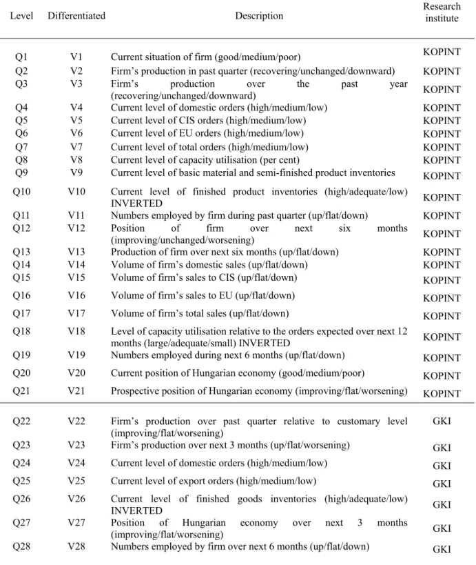
Table 1 Description of questions asked by the business survey

Level Differentiated Description Research

institute

Q1 V1 Current situation of firm (good/medium/poor) KOPINT

Q2 V2 Firm’s production in past quarter (recovering/unchanged/downward) KOPINT Q3 V3 Firm’s production over the past year

(recovering/unchanged/downward) KOPINT

Q4 V4 Current level of domestic orders (high/medium/low) KOPINT

Q5 V5 Current level of CIS orders (high/medium/low) KOPINT

Q6 V6 Current level of EU orders (high/medium/low) KOPINT

Q7 V7 Current level of total orders (high/medium/low) KOPINT

Q8 V8 Current level of capacity utilisation (per cent) KOPINT

Q9 V9 Current level of basic material and semi-finished product inventories KOPINT Q10 V10 Current level of finished product inventories (high/adequate/low)

INVERTED KOPINT

Q11 V11 Numbers employed by firm during past quarter (up/flat/down) KOPINT Q12 V12 Position of firm over next six months

(improving/unchanged/worsening) KOPINT

Q13 V13 Production of firm over next six months (up/flat/down) KOPINT

Q14 V14 Volume of firm’s domestic sales (up/flat/down) KOPINT

Q15 V15 Volume of firm’s sales to CIS (up/flat/down) KOPINT

Q16 V16 Volume of firm’s sales to EU (up/flat/down) KOPINT

Q17 V17 Volume of firm’s total sales (up/flat/down) KOPINT

Q18 V18 Level of capacity utilisation relative to the orders expected over next 12

months (large/adequate/small) INVERTED KOPINT

Q19 V19 Numbers employed during next 6 months (up/flat/down) KOPINT Q20 V20 Current position of Hungarian economy (good/medium/poor) KOPINT Q21 V21 Prospective position of Hungarian economy (improving/flat/worsening) KOPINT Q22 V22 Firm’s production over past quarter relative to customary level

(improving/flat/worsening) GKI

Q23 V23 Firm’s production over next 3 months (up/flat/worsening) GKI Q24 V24 Current level of domestic orders (high/medium/low) GKI

Q25 V25 Current level of export orders (high/medium/low) GKI

Q26 V26 Current level of finished goods inventories (high/adequate/low)

INVERTED GKI

Q27 V27 Position of Hungarian economy over next 3 months

(improving/flat/worsening) GKI

Q28 V28 Numbers employed by firm over next 6 months (up/flat/down) GKI