As a final application of the self-consistent RDLM theory, the rare earth hcp-Gd is investigated. Because Gd is in the center of the f block, Gd has a half-filled 4f shell, consisting of a localized band, energetically well separated from the delocalized conduction band.
Multiple scattering theory
Using these two types of quantities, the Green's function and the representation of the SPO can be pieced together. Entering the free particle Green's function, Eq. 1.1.23), in the definition of the structural Green's function, Eq.
Relativistic disordered local moment theory
Note that each term in Eq. 1.2.18) depends on the orientation of the local moments through the densities. We also note that in our implementation of the self-consistent RDLM scheme, the order parameter.
Spin models
Classical spin Hamiltonian
1.3.1) is the most general function (considering time-reversal symmetry) down to second order in spin components, and also corresponds to a second-order expansion of the energy in spin-orbit interaction strength forces, from a perturbation approximation. Generalizations of this second-order pair interaction model can be given both by introducing higher-order pair interactions and by allowing multi-spin interactions.
Relativistic torque method
The mapping to a classical spin model is available through the same second derivatives of the spin model, Eq. For example, if the reference system is FM and is magnetized along the z-axis, then so are the specific two-site second derivatives of the spin model.
Spin-cluster expansion
It should be noted that we have only done a special regrouping of the basic functions. Thanks to the method of extension, the terms in the summation for n-spin clusters α now depend exactly on n spins of the whole system. As in the previous cases, orthogonality of the spherical harmonics implies that only the last term of Eq.
Although on paper more concise in its final form, the logarithm in Eq. 1.3.43) is actually calculated in terms of the power series. All that remains is to map the SCE in the usual form of the spin Hamiltonian, i.e. a second-order tensorial Heisenberg model as seen in Eq. 1.3.1), determine the relationship between the two sets of infinite coefficients (leading, in general, to an infinite system of linear equations connecting the two sets of coefficients), then remove the unnecessary coefficients beyond the tensorial Heisenberg model.
We have now arrived at the final form of the tensor exchange coupling within the SCE-RDLM scheme: 1.3.47).
LSDA+U approximation
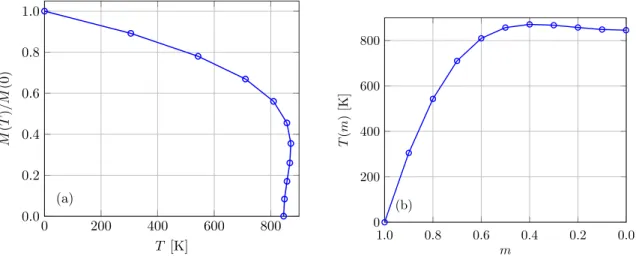
The reason for this is the non-monotonic behavior of the T(m) curve shown in the figure. The presence of the surface leads to significant changes in the electronic structure of the final layers compared to the bulk. To obtain quantitative evidence for the influence of Heisenberg terms on the spin configuration shown in Fig.
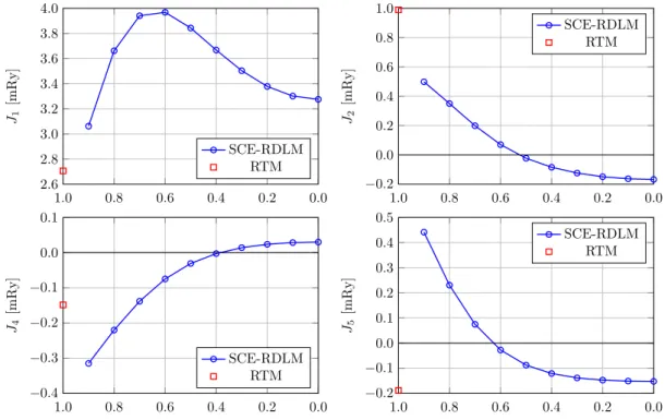
The lattice Fourier transform of the spin structure obtained for the experimental geometry is shown in Fig. From the point of view of SCE, a second-order (four rotation) SU(2)-invariant set. The red symbols show the two limits of common methods: Ground state RTM and paramagnetic SCE-RDLM.
In the current version of the program, the implicit equation for the inverse temperature (Eq.
Results 46
Fe bulk
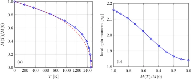
This overestimation of the temperature scale is a direct result of the mean-field approximation inherent in RDLM theory. The fact that the magnitude of the Fe moment varies so much with temperature in itself suggests that a Heisenberg model could only provide an approximate description of its behavior. One could try to correct the shortcomings of the simple Heisenberg model by explicitly incorporating some temperature dependence into the model itself.
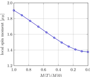
33] tried this using temperature-dependent spin model parameters, and found that the dominant nearest-neighbor effective interactions increase as the average magnetization decreases, which may explain the deficiency of the magnetization as predicted from the fixed-coupling Heisenberg model in Fig. We tried to find some hints about the origin of this feature in the magnetization dependence of the local moment, shown in Fig.
It is possible that a more careful evaluation of the temperature in the program could affect this inconsistency, indicating the need for further development of the code.
FePt bulk
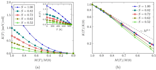
In our convention, the z direction is parallel to the c -axis of the L10 structure (expected to be the easy axis from previous work), and the x -axis is directed toward the first nearest neighbors in planes normal to the thec axis. At finite temperatures, a power-law dependence of the MAE on magnetization was found, with an exponent of about 2–2.1 over a wide temperature range [18,22], consistent with experiments [20,21]. By considering chemical and temperature-induced orientational disorder simultaneously in a consistent procedure, we can elaborate our theoretical understanding of anisotropy in FePt.
Note that the temperature-dependent part of the electronic free energy, ∆Fel(η, T) (Eq.) has a small contribution to the MAE, so we neglected it from the present calculations. To calculate the DOS accurately, we used up to 5000k points in the irreducible wedge of the BZ. This is clear if one considers the range of T5 in → the case of T5 in → the case of T5. magnetization along x the magnetizations of the two conditions become different, which implies that they cannot be described by the same probability density.
20], the shape of the symbols in that figure is matched in tone for similar values of chemical disorder.

FeRh bulk
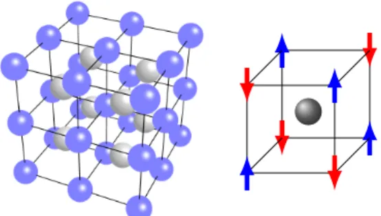
Although mostly not necessary for the construction of the phase diagram, we performed self-consistent field calculations over the entire temperature range of the FM and AFM phases for several values of the lattice constant. Note that the (induced) Rh moments are zero in the AFM phase due to symmetry, and in this phase "magnetization" refers to the magnitude of the sublattice (or staggered) magnetization. This feature together with the monotonic dependence of the Rh moment on the magnetization in the FM phase (and especially its disappearance in the PM limit) clearly confirms the induced nature of the Rh moments.
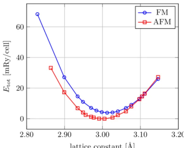
The considerably larger size of Fe moments compared to the FePt case (see Fig. 2.6) is due to the much larger Fe-Fe interatomic distance in this case - reasons arising from the electronic structure (hybridization) are refuted by the great similarity of the FM and AFM curves. Calculations of the total energy at zero temperature (see Figure 2.11) provide us with the relative stability of the FM and AFM phases at zero temperature; one point in the phase diagram. This is a manifestation of the FeRh metamagnetic phase transition provided by our RDLM theory.
To find the metamagnetic transition line of the phase diagram, we calculated the RDLM free energy curves as a function of temperature (see Eq.
Gd bulk and surface
The spin splitting of bulk states in the PM phase is somewhat more difficult to quantify with the above measures. In the PM phase, the total spin-magnetic moment is reduced to 7.41 µB, which means that a significant polarization of the conduction band still persists. It is the asymmetry of the spectral weights in the two spin channels that results in a significant conduction band moment.
This feature is slightly more pronounced in the PM phase than in the FM phase. The surface states in the FM phase near the Fermi energy are highly of majority spin character. On the other hand, in the PM phase the magnetization increases slightly to 7.48µB on the surface.
It is the asymmetry of the spectral weight for the two spin channels that accounts for the finite residual local moment of the conduction band in the PM phase, suggesting non-Stoner behavior.

Fe 1 /Rh(001) thin film
- Self-consistent field calculations
- Validity of the spin model
- Exchange interactions
- Spin dynamics simulations
For an ideal, unstrained geometry, the first nn FM isotropic Heisenberg terms dominate the energy of the spin system. We see that close to realistic geometries, the isotropic biquadratic couplings are of the same magnitude as the bilinear terms. For the experimental-9% relaxation, the damping of the first nn FM coupling is fulfilled by.
The spatial modulation of the preferred spin configuration from the Heisenberg tensor terms alone can be inferred from a mean-field evaluation. The shift of the ground state from the Γ point can be attributed to the second and third nn AFM isotropic Heisenberg couplings. It should now be noted that the mean-field estimate contains explicitly only bilinear terms of the spin model.
This is a clear indication of strong isotropic quadratic interactions dominating the bilinear part of the spin model.

Attempts to extract exchange interactions at finite temperature
- SCE-RDLM method below the Curie temperature
- The RTM-RDLM approach
However, observing the decomposition of the Green's function (and equivalently, the scattering path operator) with the real-space distance, we note that the largest contribution comes from the thek = 1 term (corresponding to the simplified pairwise interactions of the SCE-RDLM method), from which. The interactions go to zero at the Stoner-Curie temperature indicating the collapse of the local momentum. In the framework of the so-called two-temperature model (2TM) the electron temperature and the lattice (phonon) temperature are assumed to be separate but coupled quantities.
At a given time step, the spin model is selected according to the current value of the electron temperature and the instantaneous average magnetization of the simulated sample. As an alternative, we also developed a formulation of RTM in a temperature-limited RDLM state. The capabilities of the self-consistent RDLM theory go beyond the applications in this thesis.
I used the new code to investigate the variation of magnetization and local torque of bcc-Fe with temperature. I found a 15% decrease in the moment of Fe from the ferromagnetic (FM) ground state to the high-temperature paramagnetic (PM) state, indicating a limited stiffness of the Fe moment in the bulk. Therefore, I suggested that the results obtained by the RDLM method should be interpreted on the basis of average magnetization rather than temperature.