It all started from the need, on the part of the ARCHiVe center (Cini Foundation's digital artefact preservation laboratory), for a new automated system for the downstream processing of images of scanned object products, with the aim of publishing them. in the Foundation's digital library. The photos, although taken in the best possible reproducible environment, are sometimes imperfect as they do not guarantee 100%, for example, the presence of the original colors (altered by imperfections in the lights).
Cini Foundation and ARCHiVe
The foundation's initial projects were focused on solving some of the pressing problems that plagued Italy and Venice in the postwar period. The ARCHIVe Center (analysis and recordings of cultural heritage in Venice), founded in 2018 by the Giorgio Cini Foundation, the Factum Foundation for Digital Technology in Conservation and the Digital Humanities Laboratory of the 'Ecole Polytechnique F'ed'erale de Lausanne (EPFL-DHLAB), was born with the aim of paying particular attention to the development and use of new technologies for digital preservation and for the improvement of the enormous heritage present on the island of San Giorgio Maggiore in Venice, but not just not. .

Text Recognition
Moreover, there are almost no methods in the field of Optical Character Recognition (OCR) that are applicable to the language written in cuneiform. The selected workflow merges retro-digitized tracings and native digital tracings, as well as 3D scanned grids of cuneiform plates.
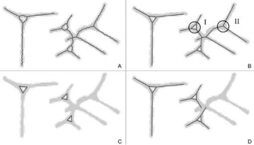
Image Classification
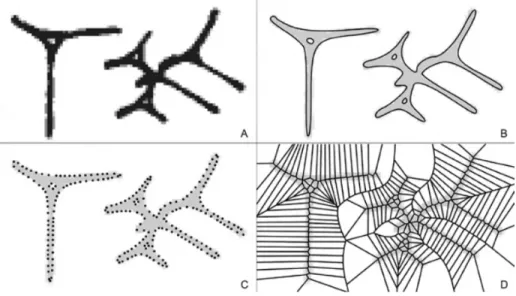
A histogram representing the count of each visual word is then computed as a global descriptor for each glyph. A higher threshold indicates that fewer glyph pairs are considered visually similar, resulting in fewer edges in the graph.
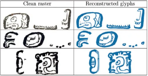
Image Processing
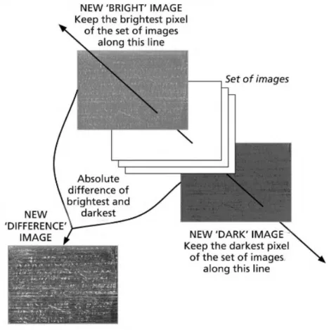
The digitization of such artifacts is the first step in the development of document interpretation. Experts who have access to the actual tablet they intend to transcribe have developed a very specific and intuitive strategy to improve the visibility of the notches left by the pen in the wood.
Neural Network
Images
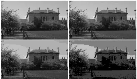
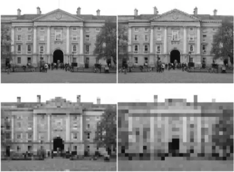
The number of samples in an image limits the objects that can be distinguished/recognized in the image. Once the cumulative distribution has been determined, we can calculate a noise value for each pixel in the image.
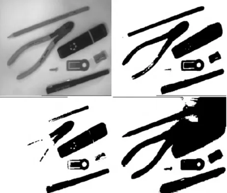
Binary Vision
In general, these transformations require some logical operation/test to be performed at each location in the image. Arguably, the most important thing to note about binary imaging is that the foreground and background being separated must be separate in the image that thresholds. However, even in the 'correct' thresholded binary image there are some errors (e.g. much of the pencil tip is missing and the shadow over the highlighter pen is incorrectly included).
Morphological operations work by performing a logical test on all possible places in the image between the structural element and the corresponding part of the image. In other words, the structuring element is effectively translated to every possible position in the image, a logical operation is applied (comparing the structuring element to the image in some way), and the result is stored in a separate output image. Binary images are treated as 2D arrays, where object points are the points in the arrays.
X⊖B={p∈ϵ2;p=x+b∈X for everyb∈B} (12) A point p is an element of the eroded output set if, and only if, that point is a member of the input image set X , when translated by each (and all) of the structuring element points/vectors b. It can also be thought of as a matching problem, where the structuring element is compared to the input image in all possible places, and the output is marked only where the structuring element and the image match perfectly. An aperture removes noise (ie, eliminates image detail smaller than the texture element), narrow features (such as bridges between larger groups of points), and smoothes object boundaries.
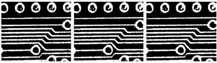
Edges
Note that one of the traces (bottom center) of the printed circuit board broke during the opening, which may indicate a problem with the board. There are many techniques in both edge-based vision and region-based vision, all of which aim to determine the best representation of the scene in terms of edges or regions. This technique is referred to as non-maxima suppression, which uses the gradient and orientation information to determine which edge points are central (i.e., the main response at each point along an edge contour).
It does this by using the orientation information from each point to determine which points are on either side of the current edge point, and then suppresses the current point if its gradient is less than either of its two neighbors. Laplacian of Gaussian: Laplacian of Gaussian is another derivative edge detector and is still one of the most widely used. The smoothing filter must meet two criteria: (1) that it is smooth and band-limited in the frequency domain (i.e. it must limit the frequencies of edges in the image) and (2) that it exhibits good spatial localization (i.e. the filter must not move the edges or change their spatial conditions).
Estimate the edge normal direction (i.e. orientation) using the first derivative of the refracted Gaussian image;. This is done by looking for zero crossings in the second derivative of the direction of the refracted Gaussian image, where those derivatives are obtained with respect to the orientations of the edges that were calculated in the previous step;. The edge gradient is calculated based on the first derivative of the Gaussian refracted image;.
Machine Learning
- Exploration of a CNN
- Architecture
- Regularization
- Optimization
- Data manipulation
In the field of ML, DL, due to its considerable success, is currently one of the most prominent research trends. The convolutional neural network (CNN) is one of the most popular and widely used DL networks. Fusion Layer: The main task of the fusion layer is to sub-sampling the feature maps.
Loss functions: The final classification is achieved from the output layer, which represents the last layer of the CNN architecture. This leads to a reduction in network parameters, which speeds up the training process and, as a result, makes it possible to solve the problem of overfitting. Then, the model results are compared to the actual, observed values of the target variable to determine accuracy.
Then the parameter is updated in the opposite direction of the gradient to reduce the error. In the third method, simulated data can be considered to increase the volume of the training set. Realizing augmentations in the color space of the channels is an alternative technique that is extremely feasible.
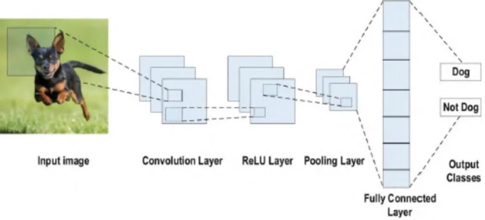
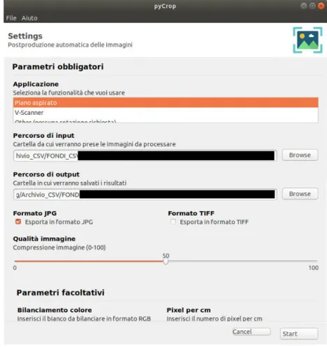
Image Postprocessing
A selection of the tool used for the original image capture is necessary, as according to the selected tool we determine the rotation the image will perform. We can now apply different filters and we just have to pass the image and the size of the kernel [14]. An additional step is represented by the compression of the images, often useful in the case of thumbnails or images of secondary importance, for which it is not necessary to maintain a high quality.
White balancing, one of the user-defined options of the application, is a process that leads to the adjustment of the intensity of colors on the basis of a. However, for this option to work, a prior installation of RawTherapee is required, as applying the color profile is done by calling the software via CLI (Command Line Interface);. It is simply a numerical value in pixels (one for each side) that can be positive or negative, and therefore corresponds to an addition or removal of part of the image.
The last practical feature, but not linked to the image processing process, is the possibility of allowing, for each processed image, a viewer to view the different steps to which it is subjected. In the meantime, it is certainly possible to broaden our horizons and try to look beyond the processes currently under consideration, further expanding the potential of the application. Another proposal under consideration concerns image straightening, that is, “straightening” the image perpendicular to the axes of the plane.
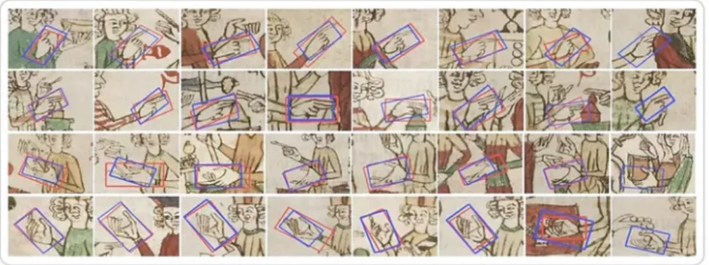
Features Detection
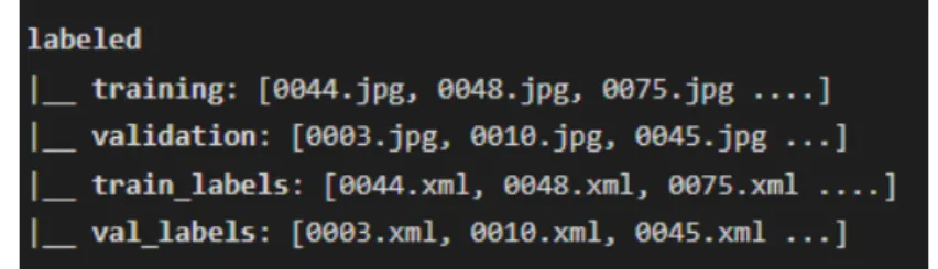
This subdivision is performed to allow the model to train on a part of the images (it is normally advisable to use about 80% of the total images in training), to then test the results of your training on unpublished images to go, never seen before. The role of the optimizer is to measure how well our model predicted output is compared to true output. In the case of the Image Classification model, after 10 epochs the validation accuracy (thus the capacity of our model to classify never-before-seen images) on average on 10 folds does not go higher than 71%.
At the end of the process, our model will be ready and we will be able to ascertain its accuracy based on the cross-test performed with the validation database during the training phase. One of the most important elements in the analysis phase of the model was represented by its level of accuracy. As for the post-production of the images, the system may seem rather heavy, but quite accurate (an estimate is between 85 and 90% accuracy), which however may seem inadequate in large numbers (from 25000 images over 2500 will be wrong, a significant number anyway).
In order to process as much as possible correctly, it is necessary to adjust the code so that the application can correctly distinguish the different parts of the image. It will be essential, although objectively useless for our acquisitions, to indicate the presence of the latter, to prevent the model from being able to confuse this element with the object we want to extract. Keeping the Revolution Going: Proceedings of the 43rd Annual Conference on Computer Applications and Quantitative Methods in Archeology (2015).
In: Proceedings of the 28th Annual Conference on Computer Graphics and Interactive Techniques (2001). Deep residual learning for image recognition.” In: Proceedings of the IEEE Conference on Computer Vision and Pattern Recognition (2016).