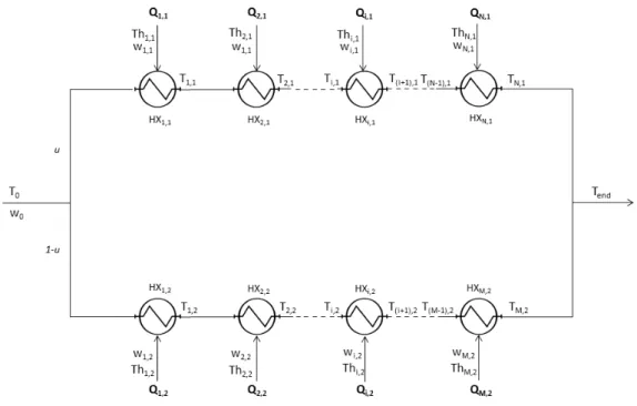
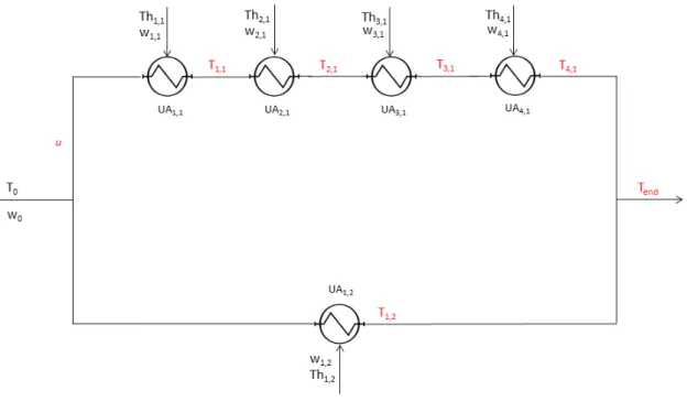
Optimal Operation of Parallel Heat Exchanger Networks - NTNU

The Jäschke temperature approach aims to achieve near-optimal operation of parallel heat exchanger networks solely by manipulating the bypass selection - based solely on simple temperature measurements. Figure 2.1 shows a simplified general heat exchanger network with N heat exchangers in series on the upper leg and M in series on the lower leg. Recently, Jäschke (Jaeschke 2012) derived the self-optimizing Jäschke temperature variable for the operation of heat exchanger networks.

Operation using the Jäschke temperature control variable is compared to optimal operation for several different heat exchanger networks. The most efficient way to transfer heat is through a counter-flow heat exchanger (Geankoplis 2003) shown in Figure 3.1.

Figure 2.1: A simplified general heat exchanger network with N heat exchanger in series on the upper branch (branch 1) and M heat exchangers in series on the lower branch (branch 2)

Steady state model

Approximations and Transformations

For the steady state investigation, the mass flow of the cold stream and each hot stream will also be considered constant. Approximation of the logarithmic mean temperature difference (LMTD) Application of the LMTD equation can lead to numerical challenges. If the LMTD were to be applied to a transition in which the temperature difference has different signs on the two sides of the heat exchanger, the argument for the logarithmic function would be negative, which is not permissible (Kay & Nedderman 1985).

A different and more robust approach to the LMTD was taken by Underwood (Underwood 1933) and is given as. 3.10) To avoid the numerical problems associated with the LMTD and for the robustness of the approximation, the Underwood approximation (Underwood 1933) will be used in parts of the steady-state simulations where the LMTD must be approximated. The NTU method calculates the effectiveness of a heat exchanger based on the flow rate with the limiting heat capacity.

Dynamic Model

The Mixed Tanks in Series Model

The systems would require minimal heat exchanger surface area, with minimal cost associated with heat exchange equipment. A general heat exchanger network with N heat exchangers in series in the upper branch and M heat exchangers in series in the lower branch is shown in Figure 4.1. For a heat exchanger network in Figure 4.1, consisting of N heat exchangers in series in the upper branch (j = 1) and M heat exchangers in series in the lower branch (j = 2), the cost function proposed by Jäschke is .

For the general heat exchanger network in Figure 4.1, the heat exchanger equation for a given heat exchanger is as follows. From this the overall energy balance is made with N heat exchanger in branch 1 and M heat exchangers in branch 2.

Figure 4.1: A general heat exchanger network with N heat exchanger in series on the upper branch (branch 1) and M heat exchangers in series on the lower branch (branch 2)

Jäschke Temperatures

Pi,1J Ti,1 (5.7) The same equations apply to the lower branch (j = 2) and the resulting weighted Jäschke temperature for the M heat exchangers in series on this branch is. Of these two cases, only the case with four heat exchangers in series is presented in the report. Additional simulation results are also given for the case of four heat exchangers in series in Appendix A.1.

The network of four heat exchangers in series parallel with one heat exchanger is shown in Figure 6.1. The results of optimal operation were compared with the Jäschke temperature operation and are given in Table 6.3.

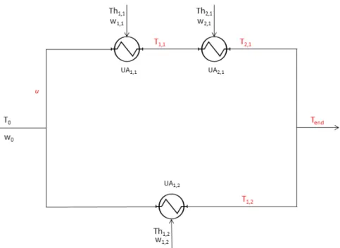
Figure 6.1: Case I: Four heat exchangers in series parallel to one heat exchanger

Case II: Two Heat Exchangers in Parallel

Jäschke Temperature Operation at Extreme Cases

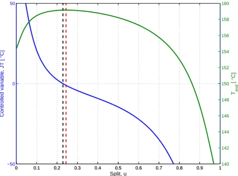
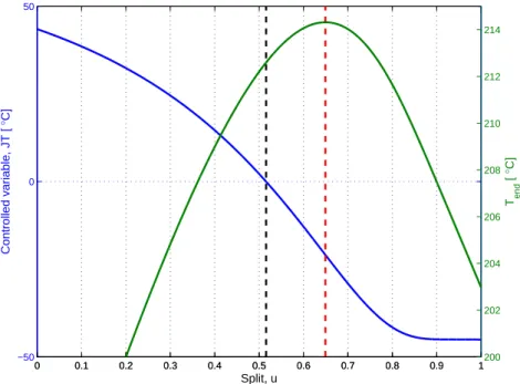
The detailed parameters for Case II-a and Case II-b are given in Tables 6.5 and 6.6 respectively. For Case II-a, this can be seen in Figure 6.4, where the control variable J T and outlet temperature Tend are plotted as a function of split u. As Figure 6.4 for Case II-a indicates, the point where J T =c1 -c2 = 0 (optimal control variable) separates differ significantly from the point of optimal operation.

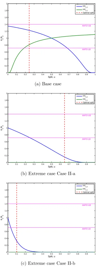
The graphs in Figure 6.6 show the relationship between θ1 and θ2 of each heat exchanger (remember section 3.1.1) with the split for the base case and both extreme cases, Case II-a and Case II-b, respectively. For case II-a, around the optimal distribution of u = 0.65, none of the heat exchangers showed a θ1/θ2 ratio within this interval.

Table 6.5: Case II-a parameters Parameter Value Unit T 0 130 [ ◦ C]

Jäschke Temperature Operaton Subject to Measurement Er-

Dynamic case II (base case): Two heat exchangers in a series-parallel heat exchanger unit. Dynamic example V: six heat exchangers in series parallel to one heat exchanger. For all networks, the parameters for each individual heat exchanger in dynamic case I–III were the same as those used in the steady state analysis in the specialization project (Aaltvedt 2012). For dynamic case IV and V, the parameters were the same as those used in the steady state analysis of this study (Section 6).

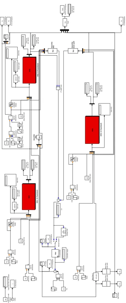
A base case, denoted Dynamic case II, of two heat exchangers in series parallel to one heat exchanger is presented in the report. The Dynamic case II heat exchanger network is given in Figure 7.1 and the complete Simulink block diagram, dynamic_21_1.mdl is given in Figure 7.2.

Figure 7.1: The dynamic case II (base case) heat exchanger network

Jäschke Temperature Operation at Small Disturbances

Both the response of the control variable (Figure 7.4) and the split response (Figure 7.5) saw a significant reduction in their overshoot and undershoot (Table 7.4) with the implementation of the analog filter. As shown by the red lines in Figures 7.4 and 7.5, the magnitude of the peaks has almost decreased to half of its original value. In Figure 7.6, it is worth noting the drop in temperature as a result of the disturbance inT h1,2 att= 1600 s.

For the cold flow passing through the upper branch, on the other hand, the temperature drop is a result of the split response associated with the disturbance in T h1,2. As can be seen in Figure 7.5, the flow split through the upper branch was increased as a result of this perturbation, eventually providing more liquid to heat, resulting in lower outlet temperatures on this branch.

Table 7.4: Analog filter parameters for Dynamic case II Filter parameter Value Unit

Jäschke Temperature Operation at Major Disturbances

The step and control variable response is given in Figure 7.7, and the resulting tuning parameters are given in Table 7.6. For both sets of tuning parameters, the modified control variable showed satisfactory system control in the presence of a cooling heat exchanger. The distribution behavior for both sets of tuning parameters is presented in Figure 7.9, which shows the distribution u as a function of time t.

This slightly different behavior can be related to the modified control variable cmod, shown in Figure 7.10. The full range of the control variable on the ordinate axis is not included in the report for readability reasons.

Table 7.5: Dynamic case II-a parameters Parameter Value Unit

Steady State Analysis Discussion

Dynamic Analysis Discussion

Heat exchanger networks with a design that allows the AMTD approach to be used in each heat exchanger are both better candidates for real large-scale processes and at the same time a configuration where the Jäschke temperature provides near-optimal operation. The observed response was far from smooth, as the bypass on the upper branch was immediately closed as Th2.1 continued to decrease below 200 ◦C (Figure 7.9). Of the modified control variable in Equation 7.1, each of the three terms includes different temperature differences.

At the point where temperature crosses are observed (Figure 7.8), violent behavior occurs as terms cancel out in the presence of zero multiplication in one given term. This makes cmod all negative and the controller will immediately close the cold flow distribution to the upper branch and thus u → 0. However, in all the cases presented in this study, the Jäschke temperature performance showed relatively close to optimal performance and good control of the system.

Also, considering the Jäschke observation of the divergent steady-state temperature of c1 6= c2 and that the control was not smooth, he still managed to operate the system satisfactorily. In the presence of smaller and more realistic perturbations, the Jäschke temperature showed tight control and good perturbation rejection for all dynamic cases studied in this report.

Further Work

For the Jäschke temperature to be versatile enough to be implemented in processes subject to such temperature fluctuations, more extensive analyzes will be required, highlighting the complexity of the heat capacity. Edvardsen (Edvardsen 2011) has shown that Jäschke's temperature control variable provided satisfactory control for a three-branch case study, using two controllers: one controlling two branches and the other controlling the third branch. Further investigations into these issues are needed for a more specific determination of the Jäschke temperature control variable and some versatility across different and more complex configurations.

Therefore, optimal operation of heat exchanger networks must include these issues, and further investigation on these topics considering the Jäschke temperature operation will be necessary. Fortunately, the Jäschke temperature includes price constants in the weighted sum in Equations 5.7 and 5.8, allowing for differently priced energy sources. In this study, the Jäschke temperature control configuration was evaluated for several different cases of parallel heat exchanger networks.

The aim was to further investigate the properties of the Jäschke temperature and determine any limitations. For the same system subject to measurement noise spanning +/−2◦C of each respective temperature, the worst case temperature loss was 3.14 ◦C. Considering the average measurement error, the Jäschke temperature showed good robustness to this kind of noise for systems with evenly distributed heat capacities. This resulted in a cooling effect, and the Jäschke temperature could not simulate the system due to singular solutions.

However, for systems with a uniform heat capacity distribution, the Jäschke temperature showed very close to optimal performance. The advantages of the Jäschke temperature control configuration are that the control variable depends only on simple temperature measurements, with split u serving as the only manipulated variable. Disadvantages of this method are the inverse response and occasional violent behavior of the control derived from Jäschke's squared measurements temperature equation.

Six Heat Exchangers in Series and One in Parallel

Subject to the equality and inequality constraints given in Section 4.1, optimal operation was determined using the built-in matlab function fmincon.

Figure A.1: The 6:1 heat exchanger network

Two Heat Exchangers in Parallel

Case II-c

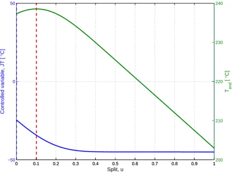
The red and black dotted lines show the optimal split with respect to the output temperature and the control variable, respectively.

Case II-d

Jäschke Temperature and Measurement Errors

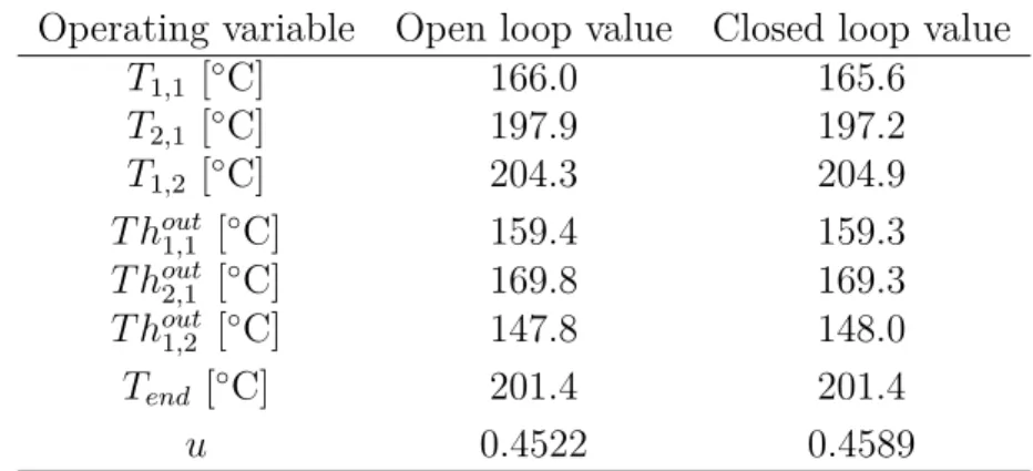
Data about the heat exchangers, which in any case apply to all heat exchangers, is given in Table B.1. Estimated heat transfer variables are given in Table B.2. Inlet parameters for the dynamic Case II are given in Table B.3. The open and closed loop outlet variables are given in Table B.5. The PI controller was tuned using the Skogestad IMC (SIMC) rules (Skogestad 2003b) for a step response of 10% increase in cold fluid mass flow.

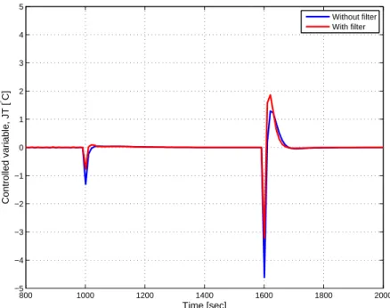
A negative step change in inlet cold stream temperature T0 of 4◦C was introduced at time= 1000 sec, and a positive step change in hot stream temperatureT h1,1 of 4◦C at time t = 1600 sec. Control variable response and split response are shown both with and without the analog filter in Figure B.2 and B.3.

Table B.1: Heat exchanger and heat transfer data Description Symbol Value Unit Total wall mass m wall 3000 [ kg ] Wall density ρ wall 7850 [ m kg 3 ] Wall volume V wall 0.3821 [ m 3 ] Heat capacity wall Cp wall 0.49 [ kg kW◦ C ] Density cold fluid ρ c 1000

Dynamic case II

Dynamic Case II-a

Dynamic Case III

The open-loop and closed-loop variables are given in Table B.11 The PI controller was tuned using the Skogestad IMC (SIMC) rules (Skogestad 2003b) on a step response of 10% increase in cold fluid mass flow rate. A negative step change in the inlet temperature of the cold stream T0 by 4 °C was introduced at time t = 1000 s, a positive step change in the temperature of the hot stream T h1.2 by 4 °C at time t = 2000 s. The response of the control variable and the split response are shown with and without the analog filter in Figures B.11 and B.12.

Dynamic Case IV

Dynamic Case V

The PI controller was tuned using the Skogestad IMC (SIMC) rules ( Skogestad 2003b ) to a step response of 10% increase in cold fluid mass flow. The Simulink block diagram is given in Figure D.6 in Section D. The control variable response and the split response are shown in Figure B.19 and B.20.