Widespread partial-depth hydrofractures in ice sheets driven by supraglacial streams

001 002 003 004 005 006 007 008 009 010 011 012 013 014 015 016 017 018 019 020 021 022 023 024 025 026 027 028 029 030 031 032 033 034 035 036 037 038 039 040 041 042 043 044 045 046

Supraglacial streams drive widespread partial-depth hydrofractures in ice sheets

David Chandler

and Alun Hubbard

1*NORCE Norwegian Research Centre and Bjerknes Centre for Climate Research, Bergen, Norway.

2Centre for Arctic Gas Hydrate, Environment and Climate, Department of Geosciences, UiT The Arctic University of

Norway, Tromsø, Norway.

3Geography Research Unit, University of Oulu, Oulu, Finland.

*Corresponding author(s). E-mail(s): [email protected];

Contributing authors:[email protected];

Abstract

Dramatic supraglacial lake drainage events in Greenland and Antarc- tica are enabled by rapid hydrofracture propagation through >1 km ice. Here, we present a slower mode of hydrofracture, where hairline surface fractures intersect supraglacial streams, and hypothesise that penetration depth is critically limited by water supply and englacial refreezing. We apply a novel model of stream-fed hydrofracture to the Greenland Ice Sheet and find that under most conditions, 2-cm-wide fractures can penetrate hundreds of metres before freezing closed. Con- ditions for full-depth hydrofracture are more restricted, requiring larger meltwater channels and/or warm englacial conditions. Given the abun- dance of streams and surface fractures across Greenland and Antarctica’s expanding ablation zones, we propose that stream-driven hydrofractures are ubiquitous – even where distant from supraglacial lakes and crevasse fields. This intriguing process remains undetectable by current satellite remote-sensing, yet has two major thermodynamic impacts that warrant further investigation. First, by driving widespread cryohydrologic warm- ing at depths far greater than surface crevassing, it explains a consistent cold bias in modelled englacial thermal profiles. Second, the associated reduction in ice viscosity and increased damage accumulation act to enhance the vulnerability of ice sheets and shelves to dynamic instability as supraglacial drainage networks expand to reach higher elevations.

1

047 048 049 050 051 052 053 054 055 056 057 058 059 060 061 062 063 064 065 066 067 068 069 070 071 072 073 074 075 076 077 078 079 080 081 082 083 084 085 086 087 088 089 090 091 092

Keywords:Ice sheet, hydrofracture, hydrology, dynamics

Abrupt supraglacial lake drainage events, driven by hydrofracture, have been reported from the Greenland Ice Sheet [1–3] and Antarctic ice shelves [4,5]. In Greenland, rapid hydrofracture has been observed to drain>10⁷ m³ of melt water through>1 km of ice in a matter of hours, driving meter-scale hydraulic uplift with distinct seismic, tectonic and dynamic signatures [1–3,6]. However, the long-term dynamic impacts of lake drainage events remain ambiguous [7–

9]. In Antarctica, lake-driven hydrofracturing is currently observed only on floating ice shelves, where it has been observed to trigger ice shelf disintegration [5,10] and, by reducing buttressing, can lead to the destabilisiation of upstream ice [11].

Here we consider a less dramatic mode of hydrofracture where thin surface fractures intersect supraglacial stream networks. During fieldwork in the abla- tion zone of the Greenland Ice Sheet [12,13], we have observed the opening of abundant hairline fractures associated with ice flow acceleration follow- ing the onset of seasonal melt (Figs.ED1-ED3). Typically, we observed sets of multiple parallel thin fractures extending hundreds of metres perpendicu- lar to prevailing ice flow, even across zones distant from crevasse fields and supraglacial lakes. The fractures were generally 1 to 2 cm wide [13] and hence remain undetectable in satellite or UAV remote-sensing observations [14]. Due to their apparent ubiquity, we propose that such surface fractures – if they can initiate hydrofractures – will have two important impacts on ice dynam- ics even if they do not all attain the bed and develop into moulins. First, the latent heat release when meltwater refreezes at depth causes englacial warming (known as cryohydrologic warming), and associated viscous softening [15–18];

and second, the fracturing itself contributes to increasing englacial damage accumulation that promotes downstream calving [19,20].

As not all surface fractures that intersect supraglacial streams develop into moulins, we hypothesise that the critical constraint for stream-driven hydrofracturing is the balance between water supply and englacial refreezing.

Water supply is limited by a combination of factors: (i) the short length of frac- ture, typically less than a few meters, underlying the stream; (ii) supraglacial channels are often choked with snow in early summer, which impedes water flow; and (iii) the hydraulic head (stream depth) driving water into an under- lying fracture is typically<2 m, whereas supraglacial lakes commonly attain depths>5 m [21–23]. Previous theoretical work suggests that surface fractures attain the bed of an ice sheet provided there is sufficient water available to maintain a full fracture [24–28]. Here we consider the dimensions of observed hairline surface fractures and supraglacial streams, and develop a model of hydrofracture propagation in cold ice where meltwater supply is limited. We apply the model to six locations on the Greenland Ice Sheet where down- borehole temperature and ice thickness measurements are available (Fig.1).

093 094 095 096 097 098 099 100 101 102 103 104 105 106 107 108 109 110 111 112 113 114 115 116 117 118 119 120 121 122 123 124 125 126 127 128 129 130 131 132 133 134 135 136 137 138 The sites are geographically constrained by the availability of boreholes instru- mented with thermistor strings, but represent a wide range of ice thickness and flow conditions in west Greenland’s land- and marine-terminating glaciers.

Stream-driven hydrofracture

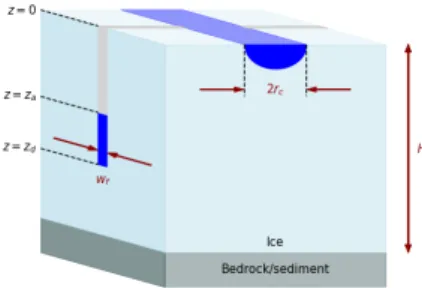
Our model calculates the downwards propagation rate of a surface fracture of lengthLf and widthwf in ice of thicknessH (Fig.2and Methods). Withzas the vertical co-ordinate (increasing downwards from zero at the ice surface), the fracture tip is at zd and the water level is at za < zd. We assume the fracture intersects a supraglacial stream with semi-circular cross section (radius rc). The model calculates fracture propagation depth using van der Veen’s [25]

linear elastic fracture mechanics, and the water filling rate due to leakage from the channel is based on Toricelli’s equation [29]. It is this leakage rate that limits fracture propagation rate. Starting with a shallow air-filled fracture, at each time step the model calculates the change in water level in the fracture, and then the new propagation depth. Refreezing by ice accretion onto the fracture walls at each level in the fracture is finally calculated following Alley et al. [26], but here we apply observed temperature profiles and the duration for which that level has been submerged. Fractures in which the accreted ice reaches the full fracture width are likely to become blocked, preventing further propagation. Therefore, blockage is more likely for thinner fractures, smaller supraglacial channels (slower leakage rate), or colder englacial ice.

We also consider two end-member cases of feedback between water flow and fracture aperture enlargement beneath the channel by viscous heat dis- sipation. In the first case we neglect any aperture enlargement, and thus implicitly underestimate meltwater supply and fracture propagation rate (the

’slow model’). In the second we use a simple treatment of this complex process, which likely overestimates aperture enlargement and fracture propagation rate (the ’fast model’). Hence, a reasonable estimate for propagation rate should lie between these two end-member limits.

Results

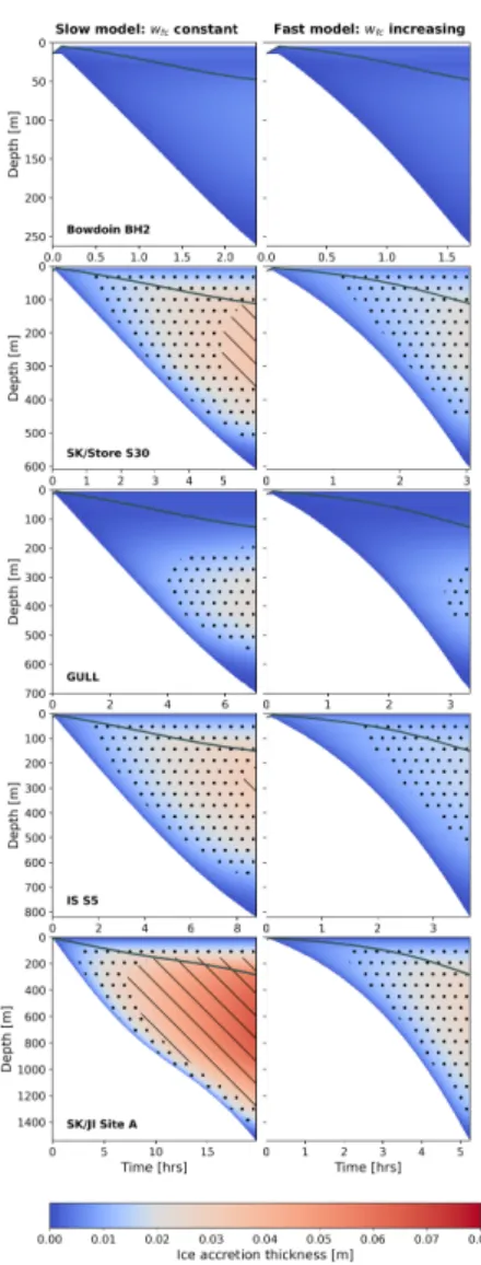
To indicate the conditions under which thin (∼2 cm) hydrofractures may become occluded by refreezing before reaching the bed, in Figs.3and4we use stippling to indicate possible occlusion (1 to 3 cm ice accretion) and hatching to indicate likely ice occlusion (>3 cm ice accretion).

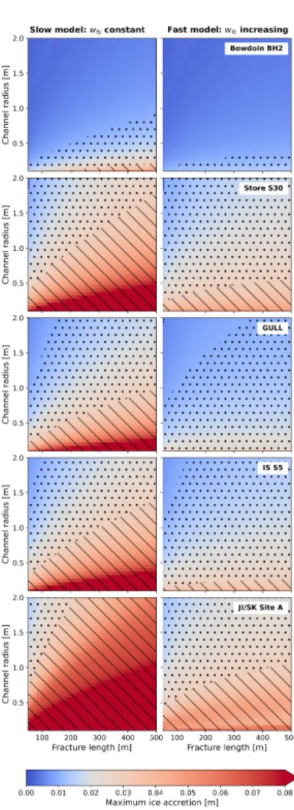
Our ’slow’ model with limited water supply demonstrates that thin frac- tures intersecting a supraglacial stream only propagate sufficiently fast to attain the bed under very restricted conditions in west Greenland. These con- ditions are site-specific, but typically require relatively short fractures or large channels (Fig. 4). A notable exception is the relatively thin, warm ice near the margin (Bowdoin Glacier BH2; Paaqitsoq GULL). Otherwise, fractures become occluded by accreting ice and are sealed shut before reaching the bed.

Both ice thickness and temperature are critical constraints on propagation

139 140 141 142 143 144 145 146 147 148 149 150 151 152 153 154 155 156 157 158 159 160 161 162 163 164 165 166 167 168 169 170 171 172 173 174 175 176 177 178 179 180 181 182 183 184

Fig. 1 Left: locations of measured temperature profiles, including those used in Figs.3and 4. The sites are: BH2 on Bowdoin Glacier [18], sites S30 and BH18c on Sermeq Kujalleq / Storeglacier (SK / SG) [30,31], GULL in the Paakitsoq region [17], Site A on Sermeq Kujalleq / Jakobshavn Isbrae (SK / JI) [32], and Site S5 on Issunguata Sermia (IS) [33].

Shading is mean annual runoff (melt and rainfall) for ice-covered regions during the period 2000 to 2019, as calculated by Collosio et al. [34] using the Modèle Atmosphérique Régional (MAR) v3.11.2 forced by ERA5 reanalysis [35]. Right: the respective temperature profiles at the borehole sites.

Fig. 2 Schematic showing key components of our model. Here a fracture of depthzd, with water levelza, is being filled by water from a supraglacial channel with radiusRc. The ice thickness isH.

185 186 187 188 189 190 191 192 193 194 195 196 197 198 199 200 201 202 203 204 205 206 207 208 209 210 211 212 213 214 215 216 217 218 219 220 221 222 223 224 225 226 227 228 229 230 depth, as demonstrated by comparison of results in Figs.3and4for SK/Store S30 and Paaqitsoq GULL (similar thickness, but SK/Store S30 is colder), or for SK/Store S30 and SK/JI Site A (similar minimum temperatures but Site A is much thicker). Fracture width is also an important constraint, with 1 cm wide fractures being far more prone to occlusion than 3 cm wide fractures: this is evident by the extensive stippled areas but more restricted hatched areas in Figs.3and4.

With our ’fast’ model that likely overestimates water supply, 1 cm wide fractures remain liable to occlusion (except at Bowdoin). However, because there is less ice accretion than with the ’slow’ model, full-depth propagation of wider (2 to 3 cm) hydrofractures is noticeably less restricted, becoming possible under most conditions. Exceptions are fractures fed by small (r_c < 0.5 m) channels at SK/Store S30 and SK/JI Site A, where the ice column is relatively cold due to rapid advection of inland ice, and is over 1000 m thick.

Assuming that hydrofracture propagation continues unimpeded until ice accretion reaches the full fracture width (indicated by the stippling and hatch- ing in Fig.3), even relatively narrow surface fractures will propagate several hundred metres before becoming choked by ice. Narrow fractures hence con- tribute to considerable englacial latent heat release (cryohydrological warming:

methods, and Fig.5) and damage accumulation even at locations where they cannot initiate moulin development. Indeed it is this scenario that is most intriguing, as the process is likely ubiquitous across Greenland’s densely frac- tured ablation zone, affecting much deeper ice than would otherwise be reached by surface crevasses, yet remaining undetected by satellite remote sensing.

With limited water supply, propagation times may be well in excess of 12 hours. During this time the channel water level is likely to have decreased from its assumed initially full level, owing to surface melt-driven diurnal changes in supraglacial stream discharge [13,36]. Accounting for this diurnal variability by assuming sinusoidal changes in leakage over diurnal time scales (see Methods), delays propagation and generally allows more ice accretion (Figs.ED5-ED6).

Interestingly, in contrast to Fig. 4 the maximum ice accretion does not nec- essarily increase monotonically with decreasingr_c and increasing L_f. This is related to the time the fracture reaches the coldest ice, relative to the times when leakage and propagation are slower. Overall the importance of diurnal variability increases for longer propagation times (e.g., in the ’slow’ model with thicker ice or smaller channels), and will likely depend on the extent to which the diurnal streamflow variability is delayed and attenuated by site-specific characteristics of the upstream supraglacial catchment [13,36].

Limitations

Our model pragmatically assumes an idealised planar fracture geometry, though at present there is little field evidence to indicate what this geom- etry should be, or how it might be affected by site-specific conditions such as basal topography. Partial support may come from structural glaciological

231 232 233 234 235 236 237 238 239 240 241 242 243 244 245 246 247 248 249 250 251 252 253 254 255 256 257 258 259 260 261 262 263 264 265 266 267 268 269 270 271 272 273 274 275 276

Fig. 3 Temporal evolution of fracture propagation and ice accretion. Fracture propagation is modelled following van der Veen [25] (see Methods). The lower edge of the shading shows the fracture depth, and the water level is shown by the solid grey line. Shading indicates the thickness of ice accretion on to the fracture walls (Eq.9), with stippling and hatch- ing indicating where total ice accretion is sufficient to close fractures of width 1 or 3 cm, respectively. These examples usedLf = 250 m,rc= 1.0 m based on observations in SW Greenland [13], and the measured borehole temperature profiles shown in Fig.1. Note that propagation rate is independent of fracture widthwf (see Methods).

observations of similar regular fractures where exposed at the margins of a polythermal glacier in Svalbard [37] and at Isungata Sermia (labeled IS S5 in Fig.1), a land-terminating outlet of the Greenland ice sheet [14]. Theoretical fracture width profiles [24,38] are not consistent with our observations, as the upper part of the fracture becomes pinched closed when water supply is limited

277 278 279 280 281 282 283 284 285 286 287 288 289 290 291 292 293 294 295 296 297 298 299 300 301 302 303 304 305 306 307 308 309 310 311 312 313 314 315 316 317 318 319 320 321 322

Fig. 4 Maximum ice accretion thickness in fractures propagating to the bed. Maximum ice accretion is an indication of the minimum fracture width needed to enable full-depth hydrofracture propagation; thinner fractures will terminate before reaching the bed. Shading indicates the ice accretion thickness (Eq.9), with stippling and hatching indicating where total ice accretion is sufficient to close fractures of width of 1 or 3 cm, respectively. These examples used the measured borehole temperature profiles shown in Fig.1.

(see Methods). The simultaneous upward propagation of basal hydrofractures [39,40] could act to decrease the timescale required to establish a full-depth fracture that connects with the subglacial drainage system, making moulin development more likely since there is less time for ice to accrete in the frac- ture. Clearly, accounting for the geometry of surface and/or basal crevasses,

323 324 325 326 327 328 329 330 331 332 333 334 335 336 337 338 339 340 341 342 343 344 345 346 347 348 349 350 351 352 353 354 355 356 357 358 359 360 361 362 363 364 365 366 367 368

and estimating if/where they are likely to intersect, would be a useful develop- ment but requires significantly more observational constraints than currently available, along with more sophisticated modelling at specific sites.

In the mid to upper ablation zone where the water supply limit becomes critical due to the colder, thicker ice, large meltwater streams are relatively sparsely distributed. However, a fracture extending laterally for some hundreds of metres will inevitably intersect other smaller channels, as well as the main channel. Indeed, multiple small moulins are frequently observed along fracture lines even in ice over 1000 m thick, and presumably connect laterally at depth in the fracture. These smaller water sources do not substantially alter the outcome of our results, since: (1) the water supplyqfrom each channel depends onr^3/2c , so smaller streams contribute disproportionately less water; and (2) at the time when the fractures are observed to open [13], many small channels are still choked with slush, and are limited in their capacity to supply water.

Surface surveys of fracture zones and early-season supraglacial stream networks would enable better estimates of the contributions from smaller channels.

Multiple cycles of hydrofracturing can potentially overcome the limitation of refreezing, and successively enable fractures to propagate more deeply. For example, if the fracture freezes closed before connecting with the bed, then released latent heat will have warmed the surrounding ice, allowing it to propa- gate further in a subsequent cycle. However, accommodating the accumulation of new ice at depth in each cycle would cause progressive widening of the surface fractures, in contrast to our observation that surface fractures remain less than∼2 cm in width rather than undergoing successive expansion [13].

Another hindrance to multiple cycles is the decreasing water level as the frac- ture propagates (Fig. 3). By the time the fracture freezes closed, the water level may have dropped almost to the point where the fracture is occluded by ice. Reopening that part of the fracture requires additional filling, allowing further refreezing below the blockage. Finally, the transient tensile stress state that induced the initial fracturing may gradually be released by viscous creep, or could even transition into compressive stress if there is moulin development and ice acceleration up-glacier [41]. Both of these scenarios act to limit the efficacy of subsequent cycles of hydrofracture.

Alternative fracture propagation models [27, 28, 38, 42] are qualitatively consistent with van der Veen [25]: specifically, dry fractures cannot penetrate to the bed, while water-filled fractures can (with the exception of shallow, nar- row water-filled fractures considered by Alley et al. [26], which cannot reach the bed). Providing that a water levelnear to the surface is required to propagate the fracture, then the process enabling that propagation is unlikely to greatly affect our results presented here, since we find that the rate and depth of prop- agation is still critically limited by water supply. Hence, unless the fracture process itself influences the geometry of the fracture, it is likely that uncer- tainties in the water filling rate rather than the choice of propagation model will act as the main source of uncertainty in our results. Nevertheless, fur- ther work to explore how irregularities in fracture geometry and ice accretion

369 370 371 372 373 374 375 376 377 378 379 380 381 382 383 384 385 386 387 388 389 390 391 392 393 394 395 396 397 398 399 400 401 402 403 404 405 406 407 408 409 410 411 412 413 414 could lead to positive feedback that generates preferential flow paths (similar to subglacial channel development from sheet flow [43]), would help to better quantify the effects of these fractures.

Implications for ice sheets

Our observations and model demonstrate the clear potential for widespread partial-depth hydrofractures, and also limited moulin development from full- depth hydrofractures, initiated by fractures that intersect supraglacial stream networks on ice sheets. This result is relevant across the extensive ablation zone of the Greenland Ice Sheet (Fig.1), extending above the equilibrium line into the wet-firn zone where hydrological controls on ice flow remain uncertain [7–

9]. In these upper regions, moulin initiation may be restricted to supraglacial lake drainage events, or to intercepts of streams much larger than those consid- ered here (e.g., Fig.ED1). This is significant due to the contrasting dynamic responses of abrupt supraglacial lake drainage events and slow/gradual moulin development from stream intercepts, and because of the sparse distribution of lakes relative to the dense network of streams.

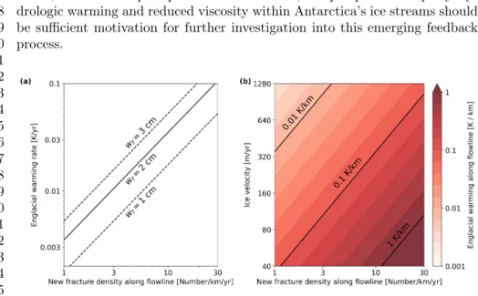
Partial-depth hydrofracturing readily explains the consistent cold bias apparent in modelled temperature profiles when compared with observations in Greenland [16,17,33,40]. Although the efficacy of cryohydrologic warming as a mechanism for ice acceleration and dynamic thinning has been argued to be limited in Greenland under present conditions [44, 45], this likely reflects an underestimate of its magnitude. For example, our results indicate that stream-driven hydrofracture will enable deeper and more widespread latent heat release than that assumed by Poinar et al.[45], where heating was limited to the upper∼300 m across regions with open crevasses. In our methods we demonstrate that resulting warming can reach 1K per 10 km along-flow even with conservative estimates for fracture density (Fig.5). Significantly, deeper latent heat release will be disproportionately more effective at enhancing ice flow, due to the nonlinear thermal-dependence and rheology of ice. Further- more, lower ice viscosity enables greater transverse strain rates, and stronger velocity gradients across shear margins, so that fast-flowing outlet glaciers and ice streams are less impeded by their margins. Therefore, as surface melting extends into the higher-elevation interior, this enhanced englacial warming potentially contributes to ice acceleration and dynamic instability in ice sheets.

Our analysis is increasingly relevant to the Antarctic Ice Sheet in a warm- ing climate. Hydrofracture has been observed to trigger ice shelf collapse [4,5,46,47], and although this is driven by surface ponding where water supply is not a limiting factor, climate warming will promote increasing melting and supraglacial stream development across ice shelves and upstream grounded ice [48,49] in a situation increasingly analogous to Greenland at present. Indeed, supraglacial drainage systems are already observed on grounded ice in West Antarctica and the Peninsula [48, 50]. Whether stream-fed hydrofractures

415 416 417 418 419 420 421 422 423 424 425 426 427 428 429 430 431 432 433 434 435 436 437 438 439 440 441 442 443 444 445 446 447 448 449 450 451 452 453 454 455 456 457 458 459 460

can stabilise ice shelves by reducing supraglacial lake volumes [51], or desta- bilise ice shelves via the latent heat and/or damage accumulation discussed above, remains an open question. Nevertheless, the prospect of deep cryohy- drologic warming and reduced viscosity within Antarctica’s ice streams should be sufficient motivation for further investigation into this emerging feedback process.

Fig. 5 Englacial warming due to latent heat released by stream-driven hydrofractures. (a) Warming ratesdTf/dtcalculated using Eq.19, which apply at depths reached by partial depth hydrofractures – perhaps several hundred metres (Fig.3), much deeper than open crevasses. (b) The cumulative effect of seemingly small warming rates in Part (a) is appar- ent when converting the time derivative to a spatial derivative (Eq.20), for representative conditions in land- and marine-terminating outlets in West Greenland. Warming scales lin- early with fracture widthwf; this plot usedwf = 2 cm.

Summary

Despite its simplicity, our model provides strong evidence that supraglacial streams are capable of driving widespread, partial-depth hydrofractures through cold ice, under a wide range of conditions representative of those encountered on the Greenland Ice Sheet – and perhaps in Antarctica under future warming. Significantly, this process is likely to be ubiquitous even out- side of regions with lakes or visible crevasses, as narrow (1 to 2 cm) fractures are abundant in the ice sheet ablation zone [13,15]. Therefore, hydrofracturing beneath streams can cause strong englacial warming in relatively thick ice (>

1 km) where full-depth hydrofractures and moulin development are dependent on lakes or unusually large channels. Noting that this mode of hydrofractur- ing will be very difficult to observe in remote sensing images, in contrast to widely-observed lake drainages [22,52–54], we clearly need more ground-based observations of the interaction between supraglacial streams and thin frac- tures. With the aid of these observations, future modelling efforts will help to constrain the magnitude of deep englacial warming or damage accumulation,

461 462 463 464 465 466 467 468 469 470 471 472 473 474 475 476 477 478 479 480 481 482 483 484 485 486 487 488 489 490 491 492 493 494 495 496 497 498 499 500 501 502 503 504 505 506 and its contribution to dynamic flow instability in Greenland and Antarctica under present and future conditions.

Methods

The downwards propagation of hydrofractures in ice sheets is similar in princi- ple to the upwards propagation of dikes in the Earth’s crust [24,26,55]. Hence, the model we develop below draws on previous work in both situations.

Van der Veen’s theory

We consider a surface fracture reaching depthdin ice of thicknessH, where the ’far field’ resistive tensile stress isR_xx(Fig. 2). Withzas the vertical co- ordinate (increasing downwards from zero at the surface), the fracture tip is atz_dand the water level is atz_a< z_d. The fracture will propagate downwards provided the elastic stress intensity factor K_I at the fracture tip exceeds a thresholdK_Ic, known as the fracture toughness [25]. In glaciers,K_Icis loosely estimated as 0.1 to 0.4 MPa^1/2 [25].

K_I is the sum of three components, corresponding to the tensile stress (K_I⁽¹⁾), ice overburden pressure (K_I⁽²⁾), and water pressure (K_I⁽³⁾). Following van der Veen [25] these are:

K_I⁽¹⁾=F(λ)R_xx√

πd (1)

K_I⁽²⁾ =−2ρ_ig

√ πd

Z zd

0

zG(γ, λ)dz (2)

K_I⁽³⁾= 2ρ_wg

√ πd

Z z_d

z_a

(z−za)G(γ, λ)dz (3) Here,Rxxis the resistive longitudinal stress [56], which is assumed constant with depth;λ=d/H;γ=z/d; and the empirical functionsF(λ)andG(γ, λ) are [25,57]:

F(λ) = 1.12−0.23λ+ 10.55λ²−21.72λ³+ 30.39λ⁴. (4)

G(γ, λ) =3.52(1−γ)

(1−λ)^3/2 −4.35−5.28γ (1−λ)^1/2 +

_{1.30−0.30γ}3/2

(1−γ²)^1/2 + 0.83−1.76γ

×[1−(1−γ)λ]

(5)

Eq.2is a simplified version of Eq. 14 in van der Veen [25], since in the abla- tion zone we assume ice density is constant with depth. For air-filled fractures (K_I⁽³⁾=0), Eqs.1and2predict that the total stress intensityKI =K_I⁽¹⁾+K_I⁽²⁾ exceedsKIc only for fractures shallower than∼20 m in a ’typical’ case (Rxx= 100 kPa,H = 200 to 2000 m). Even under an ’extreme’ high tensile stress of

507 508 509 510 511 512 513 514 515 516 517 518 519 520 521 522 523 524 525 526 527 528 529 530 531 532 533 534 535 536 537 538 539 540 541 542 543 544 545 546 547 548 549 550 551 552

R_xx= 1000 kPa, then K_I > K_Ic only for fractures penetrating ∼200 m into ice 1000 m thick. This explains why the model has predicted air-filled surface fractures cannot penetrate to the bottom of glaciers under most circumstances [58]. However, as the fracture fills with water, the higher density of water com- pared to ice allows a water-filled fracture to penetrate to the bed even in thick ice – except where prevented by refreezing [26] – consistent with predictions of other theoretical and numerical studies [26,27,42,59].

Fracture propagation through cold ice with limited water supply

As a fracture propagates downwards and its volume increases, a continued supply of water is needed to maintain a high water level. van der Veen [58]

used a simplified version of the above theory to provide a time scale for frac- ture growth under a limited (but arbitrarily specified) water supply. Since

−K_I⁽²⁾ andK_I⁽³⁾ quickly become much greater than K_I⁽¹⁾ as depth increases, the fracture propagation is controlled by the balance betweenK_I⁽²⁾ and K_I⁽³⁾. In turn, becauseK_I⁽³⁾ increases with water level in the fracture, the fracture propagation rate is effectively limited by the filling rate.

To impose the limit on water supply we consider water leaking from a channel into an initially air-filled fracture as analogous to water leaking out of a crack in a pipe. This can be estimated by Toricelli’s equation, which is commonly used in fluid dynamics to describe water leakage through small apertures [29,60,61]. For a crack of areaAin a fluid-filled pipe under hydraulic headh, the rate of fluid loss (q) is:

q=CAp

2gh (6)

The constant C lies between 0 and 1, and depends on the fluid viscosity and crack geometry. For a low viscosity fluid such as water, leaking into a transverse linear fracture,C≈0.6 [60].

Suppose a fracture of widthwf intersects a supraglacial channel (Figs.2 andED4). The fracture width is assumed to be constant with time and depth, except immediately below the channel where the width can increase to wf c

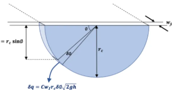
due to viscous heat dissipation as discussed below. We assume the fracture is oriented perpendicular to the channel, has a semi-circular cross section with radiusrc, and is full of water. Water depthhin the channel varies around the perimeter from 0 at the top surface torc at the bottom. In polar co-ordinates (r, ϕ) with the water surface at ϕ = 0and channel perimeter at r =rc, the total leak is the sum of many small leaks (δq) along the perimeter (Fig.ED4), i.e.,

δq=CδAp

2gh (7)

Integrating around the curved part of the perimeter (fromϕ= 0toϕ=π), using water depthh=r_csinϕand areaδA=w_{f c}r_cδϕ, we have:

553 554 555 556 557 558 559 560 561 562 563 564 565 566 567 568 569 570 571 572 573 574 575 576 577 578 579 580 581 582 583 584 585 586 587 588 589 590 591 592 593 594 595 596 597 598 q=Cw_{f c}r_c^3/2p

2g Z π

0

psinϕ·dϕ (8) The integral in Eq.8is evaluated numerically and has a value of 2.4.

Narrow fractures formed during the spring event in west Greenland can extend hundreds of metres [13]. Therefore we consider the range50≤Lf ≤500 m. The additional contribution of smaller streams intersecting long fractures is discussed as one of the limitations in the main text.

We next consider refreezing, since englacial ice in ice sheets is often well below the melting point (see temperature profiles in Fig.1). We use the Alley et al. [26] estimate for the ice accretion thicknesswi, which follows Rubin [62]:

wi(t) =2c(Tm−T0)

√πL

√

kt (9)

wherecandΓandkare the specific heat capacity, latent heat of fusion and thermal diffusivity of ice;T_mis the melting temperature; andT₀is the englacial ice temperature. Noting that ice freezes on to both sides of the fracture, the remaining open fracture width after time t is w_f −2w_i(t). Refreezing was considered briefly by van der Veen [58] using this equation, but neglected as being too slow to affect the propagation of ’crevasses’ (which are typically of order 1 m in width), unless hydrofracture to the bed takes ’several days or so’. More recent studies have also neglected refreezing [27, 42], but they also considered wide fractures (widths 0.1 to 5 m) which are a factor of 10 to 500 times wider than the observed cm-scale fractures we consider here.

Fracture width

In the model presented above we have imposed a simple fracture geometry in which the width wf is constant with depth, except immediately beneath the channel.wf is estimated using our observations of fractures at the sur- face. While the assumption of parallel-sided fractures has been shown to be reasonable for water-filled fractures [38], it may not hold for partially water- filled fractures. As an alternative we could have used the theoretical approach of Krawczynski et al. [38] (following Weertman [24]) to calculate how frac- ture width varies with depth. Taking Eqs. 3 and 4 from the supplement in Krawczynski et al. [38], we have in our notation:

wf(z) =M(πσ+ρigz)Zd−M ρwgZaZd

+1

2M ρ_igz²ln _z

d+Zd

zd−Zd

+1

2M ρ_wg(z²−z_a²) ln|Za+Zd

Za−Zd

|

−M ρwgzazln|zaZd+zZa

zaZd−zZa

|+M ρwgz²_aln|Zd+Za

Zd−Za

|

(10)

599 600 601 602 603 604 605 606 607 608 609 610 611 612 613 614 615 616 617 618 619 620 621 622 623 624 625 626 627 628 629 630 631 632 633 634 635 636 637 638 639 640 641 642 643 644

whereZ_d=p

z_d²−z²,Z_a =p

z_d²−z_a²,M = 4(1−ν)/(πµ),µandνare the elastic shear modulus and Poisson’s ratio for ice, andσis the far-field tensile stress (σ_t) modified by additional terms accounting for the fracture geometry:

σ=σ^′_x−2

πρigzd−ρwgza+ 2

πρwgzaarcsin za

zd

+2

πρwgZa (11) Although this theory has been successfully applied to supraglacial lake drainage [38], some problems arise when water supply is limited. First, unless the fracture remains almost completely water filled, a constriction develops in the upper fracture (see Fig.ED7a). When using the stress intensity approach to calculate propagation depth, the water level is too low to prevent this con- striction, which then blocks additional water flow into the fracture. If instead we impose the condition that the fracture remains completely water filled, and just use Eq.10to calculate the width at the surface (which is then a good esti- mate for the width at depth), we find the fracture steadily widens as its depth increases, soon becoming far wider than the observed cm-scale surface fractures considered here (see Fig.ED7b). Although we could conclude from this theory that deep propagation of thin fractures is not possible in cold ice – bearing in mind there is still no direct evidence of this process – it would contradict com- pelling indirect evidence, i.e., our observations of stream capture and moulin development by thin fractures, through several hundred metres of ice (Figs.

ED1-ED3). To enable moulin development without lake drainage, these thin fractures must under some conditions be able to propagate sufficiently deeply to connect with the subglacial drainage system.

The discrepancies between theoretical predictions and our observations should be explored further in future studies. For now we adopt the simple assumption that the fractures we observe are parallel-sided with a width that is constant in time. The one exception we consider is widening of the very top of the fracture by viscous heat dissipation, which we estimate next.

Viscous heat dissipation and drag

Viscous heat dissipation released as the water loses height in the fracture will cause some melting of the ice walls, and will exert drag that limits the water velocity.

In the water filled part of the fracture, we assume a steady vertical water velocity and assume that loss in gravitational potential energy is dissipated locally. From conservation of energy, the total wall melt at depth z for a fracture that has penetrated to depthz_d (withz_d> z > z_a) is:

w_m= ρwgwf

Γρ_i (z_d−z) (12)

where Γ is the latent heat of fusion of ice. Eq. 12 predicts less than 1 mm of melt for a fracture 2 cm wide penetrating the full depth of ice 1000 m thick, so it is unlikely to make an important contribution if the melt is distributed evenly. The case of preferential flow paths developing in partially

645 646 647 648 649 650 651 652 653 654 655 656 657 658 659 660 661 662 663 664 665 666 667 668 669 670 671 672 673 674 675 676 677 678 679 680 681 682 683 684 685 686 687 688 689 690 ice-choked fractures is not considered here. Of course, viscous heat dissipation does eventually need to become important if a moulin shaft is to develop (as illustrated in the cases shown in Extended Data Figs.ED1andED2). In the air-filled upper part of the fracture, the aperture in the channel floor should widen quicker than the wall melting rate estimated in Eq.12, because water flow is concentrated in the region directly under the channel rather than across the full fracture length. This process is difficult to capture in a simple model, but if we assume viscous heat dissipation is spread evenly across a length of fracture equivalent to the width of the channel (2r_c), the change in fracture width (w_{f c}) just beneath the channel is estimated as:

dw_{f c}

dt = qρ_wg 2rcΓρi

(13) However, Eq.13likely overestimates melting because (1) the water should spread laterally in a thin fracture, such that2rcis a minimum estimate; and (2) aswf c increases, the fracture walls exert decreasing resistance to water flow, so that the lost potential energy is increasingly used to accelerate the water locally, before eventually being dissipated at a greater depth. For now, we consider two end members: the ’slow’ model which excludes any moulin growth below the channel (i.e., dwf c/dt = 0), and the ’fast’ model which includes the (likely overestimated) moulin growth in Eq.13. In future, more elaborate models should certainly consider the processes of water flow and viscous heat dissipation in more detail, using computational fluid dynamics rather than our simple empirical approach.

As well as water supply rate, fracture propagation rate could be limited by the vertical water velocity in the fracture iself. Indeed, this limits propagation rate in the Alley et al. [26] model. In a vertical, parallel-sided fracture, the water flow rateQ(equivalent to the vertical water velocity in m s⁻¹) in their model is:

Q=Gw³_f

12η (14)

where η = 1.8×10⁻³ Pa s is the water viscosity and G is the hydraulic potential gradient. For steady vertical flow in the fracture, away from the crack tip, we can use the approximationG=ρwg. This would giveQ= 0.5 to 4 m s^-1 in a fracture of width 1 to 2 cm. Therefore, given that full-depth fracture propagation takes over an hour even in thin ice (propagation rate << 0.1 m s^-1: Fig.3), our results suggest it is the water supply to the crack rather than viscous drag within the crack that limits propagation rate of fractures beneath supraglacial streams. We reach this different conclusion to Alley et al.

[26] partly because of our imposed limit on water supply, and partly because we specify fracture widthwf directly (based on our observations) rather than following their approach of calculating wf using the elastic properties of ice, which initially yields much thinner fractures that are more prone to occlusion (see Eqs 1 to 4 in Alley et al. [26]).

691 692 693 694 695 696 697 698 699 700 701 702 703 704 705 706 707 708 709 710 711 712 713 714 715 716 717 718 719 720 721 722 723 724 725 726 727 728 729 730 731 732 733 734 735 736

Numerical solution

Now we can estimate the propagation and refreezing rates of a hydrofracture driven by supraglacial channel leakage. For propagation, van der Veen [58]

used the approximation

dzd

dt = ρw

ρi

2/3

Q (15)

whereQis the filling rate (in m/hr), here equivalent toq/(L_fw_f). Although this yields an excellent approximation forz_d, we use the full solution (Eqs. 1 -3) because we also want to track the upper water level when estimating ice accretion.

We assume that fractures are initially air-filled (z_a =z_d), and have already propagated to the maximum depth given by the condition K_I > K_Ic. This depth,d₀, is evaluated numerically using Eqs.1and2. We note that bothR_xx andK_Ic are poorly constrained. We have considered the respective ranges 50 to 500 kPa and 0.1 to 0.4 MPa m^1/2, but find very little sensitivity to these choices. All reported results used 100 kPa and 0.2 MPa m^1/2.

The fracture tip and water level are at z_d(t)and z_a(t), respectively (Fig.

2). Starting with an empty fracture (z_d(0) =z_a(0) =d₀), we add water to the fracture at rateq. The change in water level is:

dz_a dt =dz_d

dt − q Lfwf

(16) Eq.16is integrated numerically; at each time step, the new fracture depth zd is first evaluated using the stress intensities and current water level (Eqs.

1 - 3), before calculating the new water level. In the ’slow’ model q is held constant, and in the ’fast’ modelqincreases aswf c increases according to Eq.

13.

Similarly to Alley et al. [26] we do not couple water flow and ice accre- tion. Therefore, the ice accretion is calculated separately, using the cumulative time for which each level z has been between zd and za. We then evaluate likely propagation depth by comparing the accreted ice thickness with typical fracture widths, as indicated by the stippling and hatching in Figs.3and4.

Interestingly the fracture propagation rate is independent of fracture width wf in both models. In the ’slow’ model, water supply rateqis proportional to wfc(from Eq.8), but we maintainwf =wf c, cancellingwf in the denominator of Eq.16. In the fast model where we also consider widening of the top of the fracture by viscous heat dissipation, the change in fracture width just below the channel (wf c) is given by Eq.13. Takingwf c=wf att=0, Eq.13is solved to give

wf c(t) =wfe^αt (17)

where α contains other constants and parameters from Eqs. 8 and 13.

Hence, by substitutingwf c for wf in the expression for q (Eq. 8), we again

737 738 739 740 741 742 743 744 745 746 747 748 749 750 751 752 753 754 755 756 757 758 759 760 761 762 763 764 765 766 767 768 769 770 771 772 773 774 775 776 777 778 779 780 781 782 find thatw_f cancels from Eq.16. However, while the propagation rate is inde- pendent ofw_f, the time taken to occlude the fracture by freezing (and hence, the likely propagation depth), and the strength of englacial warming (below), are both sensitive to this parameter.

Englacial warming

One potentially important consequence of hydrofractures, besides moulin development, is their potential to cause englacial warming. This is relevant whether or not the fracture reaches the bed, provided the water refreezes locally before draining out. Here we use a straightforward energy balance cal- culation to estimate warming under a range of relevant conditions (fracture densities and ice flow velocities). We consider the along-flow fracture density Df (units: number per km per year), which is the number of fractures forming each year per unit length along a surface flow line. We have few constraints on Df, except at moulin L41 where we have observed Df ≥ 13 km⁻¹ yr⁻¹ (surface velocity∼0.15 km yr⁻¹; at least 2 new sets of fractures each year; so locallyDf ≥2/0.15 = 13km⁻¹yr⁻¹). If all the water filling the new fractures refreezes, then the equivalent volume-averaged englacial heat sourceQf (in J m⁻³ yr⁻¹) is:

Qf =DfwfρwΓ (18)

The rate of englacial warming (in K yr⁻¹) due to the fractures is then dTf

dt = Qf

ρ_ic_p =D_fw_fρw

ρ_i Γ

c_p (19)

This warming applies at all levels above the lower limit of fracture propaga- tion. Although these rates appear small (Fig.5a), their effectiveness is more apparent if considering typical flow velocities, and the many decades taken to advect ice through the ablation zone. For ice velocityV, the rate of englacial warmingper unit distance along the flow direction, i.e. in the Lagrangian sense,

is: dTf

dx = 1 V

dTf

dt (20)

Given that the ablation zone is tens of km across in west Greenland, warming of several K appears reasonable even with quite a low density of new fractures (Fig.5b). For example, withV in the range 100 to 200 m yr⁻¹, warming of 1 K per 10 km could be achieved with a fracture density of 3 to 6 km⁻¹ yr⁻¹.

Diurnal variability

When calculating leakage rate (Eqs8) we have assumed that the supraglacial channel remains full. This is a reasonable assumption considering that audi- ble fracturing is more prevalent during the evening [13], associated with hydrologically-driven ice acceleration [13,63]. However, because hydrofractures can take>12 hours to attain the bed (Fig.3), the effects of reduced channel water levels should be considered. Clearly this is very dependent on specific

783 784 785 786 787 788 789 790 791 792 793 794 795 796 797 798 799 800 801 802 803 804 805 806 807 808 809 810 811 812 813 814 815 816 817 818 819 820 821 822 823 824 825 826 827 828

catchment size and hypsometry, snow remnants, etc., but an estimate provides some interesting insight. Suppose the water depth at the channel centre varies from a maximumr_c (late afternoon) to a minimum 0.5r_c (morning). For this half-filled channel the water level extends across the channel from ϕ = π/6 to ϕ = 5π/6. Hence, for minimum leakage the integral in Eq. 8 would be R5π/6

π/6

√sinϕ−0.5dϕ= 1.15instead of Rπ 0

√sinϕdϕ= 2.40. If this represents the range of a sinusoidal variation in leakage, we can run the model with Eq.

8replaced by

q=Cwfr^3/2_c [1.78 + 0.63 cos(2πt)] (21) where time t has units of days. In this case the reduced leakage delays propagation sufficiently to make a noticeable increase in ice accretion (Figs.

ED5-ED6). Characterising the temporal variability in stream flow should be worthwhile if applying this model to specific sites.

829 830 831 832 833 834 835 836 837 838 839 840 841 842 843 844 845 846 847 848 849 850 851 852 853 854 855 856 857 858 859 860 861 862 863 864 865 866 867 868 869 870 871 872 873 874 Acknowledgments. DC acknowledges support for fieldwork from UK NERC grant NE/H023879/1. AH gratefully acknowledges a research profes- sorship from the Research Council of Norway through its Centre of Excellence funding scheme (SFF Grant 223259), Arctic Interactions funding from the Uni- versity of Oulu and the Academy of Finland (PROFI4: Grant 318930) and an Arctic Five Professorship. Field observations were kindly supported by The Royal Geographical Society (Walters Kundert Fellowship), the Greenland Ana- logue Project (GAP-SPB), Lars Ostenfeld / Caspar Haarløv ("Into the Ice") and James Reed / Ted Giffords (BBC "Frozen Planet II").

Author contributions

DC developed the model; both authors contributed to writing the manuscript.

Competing interests

The authors declare no competing interests.

Availability of data and materials

MAR v3.11.2 data were downloaded from ftp://ftp.climato.be/fettweis/

.MARv3.11.2/(last access: 24 June 2022).

Code availability

Python scripts for the fracture propagation model are available on request from the corresponding author.

875 876 877 878 879 880 881 882 883 884 885 886 887 888 889 890 891 892 893 894 895 896 897 898 899 900 901 902 903 904 905 906 907 908 909 910 911 912 913 914 915 916 917 918 919 920

Extended data

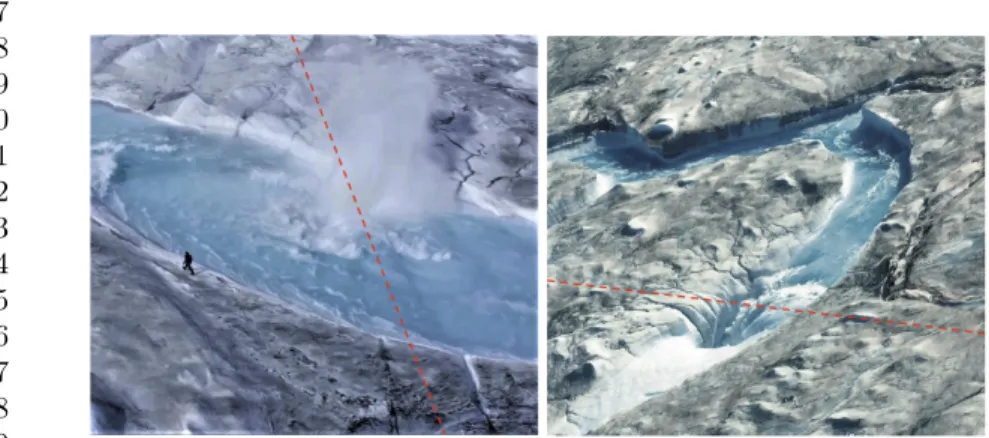
Fig. ED1 Active hydrofracture and moulin genesis where surface fractures intersected a supraglacial river on the K-Transect, West Greenland (67.124^◦N 49.298^◦W, ice thickness

∼1265 m [64,65]). The site is close to Isunguata Sermia (labeled IS S5 in Fig.1). Left: photo taken on 18 July 2019 when the fracture was observed to open with the onset of moulin formation and active stream interception. Right: photo taken on 25 July 2019, when the moulin had fully developed, and captured all supraglacial river discharge in an act of rapid glaciofluvial piracy. Red dashes show the approximate orientation of the surface fractures.

Although this specific case is for a channel larger than the maximum considered in our model experiments, it nevertheless demonstrates that full depth hydrofracture is possible from supraglacial stream interception even through thick (>1200 m) ice - consistent with a tendency towards increasing likelihood as channel radiusrc increases in Fig.4. The rate of development also demonstrates that enlargement of the fracture below the stream by viscous heat dissipation - as considered in our ’fast’ model - is a potent process that rapidly accelerates stream capture.

921 922 923 924 925 926 927 928 929 930 931 932 933 934 935 936 937 938 939 940 941 942 943 944 945 946 947 948 949 950 951 952 953 954 955 956 957 958 959 960 961 962 963 964 965 966

Fig. ED2 Fracture zone and moulin development at Leverett Catchment site L41 (ice thickness∼800 to 900 m). The site is close to Isunguata Sermia (labeled IS S5 in Fig. 1).

Here a period of audible fracturing commenced on 3 June 2012, associated with seasonal ice flow acceleration as described by Chandler et al. [13]. Left: The fracture zone developed on 3 June and extended over 1 km across-flow. Photo taken 23 June 2012; drill is∼1 m tall. Right: Moulin L41A, which developed on the same fracture zone. Photo taken 13 June 2012, approximately 10 days after fracturing. Diurnal variations in stream discharge were typically 3 to 8 m³s⁻¹. [13]

Fig. ED3 Close to the margin in the Leverett catchment (ice thickness∼400 m), where stream capture lead to the development of moulin L7 used for tracing experiments in 2011 [12]. The photo was taken 8 June 2011, 1 day after the fracture opened. The hose width is approximately 25 mm.

967 968 969 970 971 972 973 974 975 976 977 978 979 980 981 982 983 984 985 986 987 988 989 990 991 992 993 994 995 996 997 998 999 1000 1001 1002 1003 1004 1005 1006 1007 1008 1009 1010 1011 1012

Fig. ED4 Schematic showing how water leakage is calculated in Eqs.6to8. The total leak qfrom the channel into the fracture is treated as the sum of many small leaksδq(Eq.7).

Each small leak is calculated using Toricelli’s equation (Eq.6); these are integrated around the curved perimeter of the channel cross section fromϕ= 0toϕ=π(Eq.8). In the ’slow’

model, the fracture widthw_{f c} just below the channel is fixed at a constantw_{f c}=w_f (as shown in Fig.2). In the ’fast’ model,wf c increases with time close to the channel because turbulent heat transfer melts the ice where water is entering the fracture (see Eq.13), but remains fixed atwf elsewhere. Additional symbols are the parameterC in Toricelli’s equation, water depthh(ϕ), and channel radiusrc.

1013 1014 1015 1016 1017 1018 1019 1020 1021 1022 1023 1024 1025 1026 1027 1028 1029 1030 1031 1032 1033 1034 1035 1036 1037 1038 1039 1040 1041 1042 1043 1044 1045 1046 1047 1048 1049 1050 1051 1052 1053 1054 1055 1056 1057 1058

Fig. ED5 Temporal evolution of fracture propagation and ice accretion. This is the same as Fig.3, except that diurnal changes in channel water level are included. The lower edge of the shading shows the fracture depth, and the water level is shown by the grey solid line.

Shading indicates the thickness of ice accretion on to the fracture walls (Eq.9), with stippling and hatching indicating where total ice accretion is sufficient to close fractures of width 1 or 3 cm, respectively, before they reach the bed. These examples usedLf = 250 m,rc = 1.0 m based on observations in SW Greenland [13], and the measured borehole temperature profiles shown in Fig.1. Note that propagation rate is independent of fracture widthwf

(see Methods). The main changes from Fig.3are the longer propagation times, which allow thicker ice accretion and a more restricted range of conditions for full-depth hydrofracture.

1059 1060 1061 1062 1063 1064 1065 1066 1067 1068 1069 1070 1071 1072 1073 1074 1075 1076 1077 1078 1079 1080 1081 1082 1083 1084 1085 1086 1087 1088 1089 1090 1091 1092 1093 1094 1095 1096 1097 1098 1099 1100 1101 1102 1103 1104

Fig. ED6 Maximum ice accretion thickness in fractures propagating to the bed. This is the same as Fig.4, except that diurnal changes in channel water level are included. Maximum ice accretion is an indication of the minimum fracture width needed to enable full-depth hydrofracture propagation; thinner fractures will terminate before reaching the bed. Shading indicates the thickness of ice accretion (Eq.9), with stippling and hatching indicating where total ice accretion is sufficient to close fractures of width of 1 or 3 cm, respectively. These examples used the measured borehole temperature profiles shown in Fig.1.

1105 1106 1107 1108 1109 1110 1111 1112 1113 1114 1115 1116 1117 1118 1119 1120 1121 1122 1123 1124 1125 1126 1127 1128 1129 1130 1131 1132 1133 1134 1135 1136 1137 1138 1139 1140 1141 1142 1143 1144 1145 1146 1147 1148 1149 1150

Fig. ED7 Theoretical estimates of fracture widths. (a) Fracture width profiles calculated following Krawczynski et al. [38] (Eq.10) for partially-filled fractures that have propagated tozd = 800 m. This shows how predicted fracture widths are very sensitive to water level za; it also shows the development of the constriction in the upper part of the fracture, once water level starts to drop below the surface (za/zddecreasing just below 1), which prevents us applying their model to partially-filled fractures in our study. Qualitatively similar profiles are found for other reasonable values ofzdandσ_x^′. (b) Estimates of fracture widths at the surface, for completely water-filled fractures, again following Krawczynski et al. [38] (Eq.

10; blue lines). For comparison, the black line represents the observed∼2 cm-wide fractures considered in this study (grey shaded range 1 to 3 cm). Calculations used plausible tensile far-field deviatoric stresses of 50, 100 and 200 kPa (dashes, solid, dotted lines, respectively).

Although such wide surface fractures are observed following lake drainage events [1,2] they are well beyond the range of widths that we have observed to be associated with supraglacial stream capture.

1151 1152 1153 1154 1155 1156 1157 1158 1159 1160 1161 1162 1163 1164 1165 1166 1167 1168 1169 1170 1171 1172 1173 1174 1175 1176 1177 1178 1179 1180 1181 1182 1183 1184 1185 1186 1187 1188 1189 1190 1191 1192 1193 1194 1195 1196

References

[1] Das, S.B., Joughin, I., Behn, M.D., Howat, I.M., King, M.A., Lizarralde, D., Bhatia, M.P.: Fracture Propagation to the Base of the Greenland Ice Sheet During Supraglacial Lake Drainage. Science 320(5877), 778–781 (2008).https://doi.org/10.1126/science.1153360

[2] Doyle, S.H., Hubbard, A.L., Dow, C.F., Jones, G.A., Fitzpatrick, A., Gusmeroli, A., Kulessa, B., Lindback, K., Pettersson, R., Box, J.E.: Ice tectonic deformation during the rapid in situ drainage of a supraglacial lake on the Greenland Ice Sheet. Cryosphere7(1), 129–140 (2013).https:

//doi.org/10.5194/tc-7-129-2013

[3] Tedesco, M., Willis, I.C., Hoffman, M.J., Banwell, A.F., Alexander, P., Arnold, N.S.: Ice dynamic response to two modes of surface lake drainage on the Greenland ice sheet. Environ. Res. Lett.8(3), 034007 (2013).https:

//doi.org/10.1088/1748-9326/8/3/034007

[4] Scambos, T., Fricker, H.A., Liu, C.-C., Bohlander, J., Fastook, J., Sargent, A., Massom, R., Wu, A.-M.: Ice shelf disintegration by plate bending and hydro-fracture: Satellite observations and model results of the 2008 Wilkins ice shelf break-ups. Earth Planet. Sci. Lett.280(1), 51–60 (2009).

https://doi.org/10.1016/j.epsl.2008.12.027

[5] Arthur, J.F., Stokes, C., Jamieson, S.S.R., Carr, J.R., Leeson, A.A.:

Recent understanding of Antarctic supraglacial lakes using satellite remote sensing. Prog. Phys. Geogr.: Earth Environ. 44(6), 837–869 (2020).https://doi.org/10.1177/0309133320916114

[6] Christoffersen, P., Bougamont, M., Hubbard, A., Doyle, S.H., Grigsby, S., Pettersson, R.: Cascading lake drainage on the Greenland Ice Sheet trig- gered by tensile shock and fracture. Nat. Commun.9(1064), 1–12 (2018).

https://doi.org/10.1038/s41467-018-03420-8

[7] Doyle, S.H., Hubbard, A., Fitzpatrick, A.A.W., van As, D., Mikkelsen, A.B., Pettersson, R., Hubbard, B.: Persistent flow acceleration within the interior of the Greenland ice sheet. Geophys. Res. Lett. 41(3), 899–905 (2014).https://doi.org/10.1002/2013GL058933

[8] Flowers, G.E.: Hydrology and the future of the Greenland Ice Sheet. Nat. Commun. 9(2729), 1–4 (2018). https://doi.org/10.1038/

s41467-018-05002-0

[9] Williams, J.J., Gourmelen, N., Nienow, P.: Complex multi-decadal ice dynamical change inland of marine-terminating glaciers on the Greenland Ice Sheet. J. Glaciol. 67(265), 833–846 (2021).https://doi.org/10.1017/

jog.2021.31

1197 1198 1199 1200 1201 1202 1203 1204 1205 1206 1207 1208 1209 1210 1211 1212 1213 1214 1215 1216 1217 1218 1219 1220 1221 1222 1223 1224 1225 1226 1227 1228 1229 1230 1231 1232 1233 1234 1235 1236 1237 1238 1239 1240 1241 1242 [10] Leeson, A.A., Forster, E., Rice, A., Gourmelen, N., van Wessem, J.M.:

Evolution of Supraglacial Lakes on the Larsen B Ice Shelf in the Decades Before it Collapsed. Geophys. Res. Lett.47(4), 2019–085591 (2020).https:

//doi.org/10.1029/2019GL085591

[11] Scambos, T.A., Bohlander, J.A., Shuman, C.A., Skvarca, P.: Glacier accel- eration and thinning after ice shelf collapse in the Larsen B embayment, Antarctica. Geophys. Res. Lett. 31(18) (2004).https://doi.org/10.1029/

2004GL020670

[12] Chandler, D.M., Wadham, J.L., Lis, G.P., Cowton, T., Sole, A., Bartholomew, I., Telling, J., Nienow, P., Bagshaw, E.B., Mair, D., Vinen, S., Hubbard, A.: Evolution of the subglacial drainage system beneath the Greenland Ice Sheet revealed by tracers. Nat. Geosci. 6(3), 195–198 (2013).https://doi.org/10.1038/ngeo1737

[13] Chandler, D.M., Wadham, J.L., Nienow, P.W., Doyle, S.H., Tedstone, A.J., Telling, J., Hawkings, J., Alcock, J.D., Linhoff, B., Hubbard, A.:

Rapid development and persistence of efficient subglacial drainage under 900 m-thick ice in Greenland. Earth Planet. Sci. Lett.566, 116982 (2021).

https://doi.org/10.1016/j.epsl.2021.116982

[14] Jones, C., Ryan, J., Holt, T., Hubbard, A.: Structural glaciology of Isun- guata Sermia, West Greenland. J. Maps14(2), 517–527.https://doi.org/

10.1080/17445647.2018.1507952

[15] Phillips, T., Rajaram, H., Steffen, K.: Cryo-hydrologic warming: A poten- tial mechanism for rapid thermal response of ice sheets. Geophys. Res.

Lett.37(20) (2010).https://doi.org/10.1029/2010GL044397

[16] Phillips, T., Rajaram, H., Colgan, W., Steffen, K., Abdalati, W.: Eval- uation of cryo-hydrologic warming as an explanation for increased ice velocities in the wet snow zone, Sermeq Avannarleq, West Greenland. J.

Geophys. Res. Earth Surf.118(3), 1241–1256 (2013).https://doi.org/10.

1002/jgrf.20079

[17] Lüthi, M.P., Ryser, C., Andrews, L.C., Catania, G.A., Funk, M., Hawley, R.L., Hoffman, M.J., Neumann, T.A.: Heat sources within the Greenland Ice Sheet: dissipation, temperate paleo-firn and cryo-hydrologic warming.

Cryosphere9(1), 245–253 (2015).https://doi.org/10.5194/tc-9-245-2015 [18] Seguinot, J., Funk, M., Bauder, A., Wyder, T., Senn, C., Sugiyama,

S.: Englacial Warming Indicates Deep Crevassing in Bowdoin Glacier, Greenland. Front. Earth Sci. 8 (2020). https://doi.org/10.3389/feart.

2020.00065

[19] Albrecht, T., Levermann, A.: Fracture-induced softening for large-scale

1243 1244 1245 1246 1247 1248 1249 1250 1251 1252 1253 1254 1255 1256 1257 1258 1259 1260 1261 1262 1263 1264 1265 1266 1267 1268 1269 1270 1271 1272 1273 1274 1275 1276 1277 1278 1279 1280 1281 1282 1283 1284 1285 1286 1287 1288

ice dynamics. Cryosphere8(2), 587–605 (2014).https://doi.org/10.5194/

tc-8-587-2014

[20] Krug, J., Weiss, J., Gagliardini, O., Durand, G.: Combining damage and fracture mechanics to model calving. Cryosphere8(6), 2101–2117 (2014).

https://doi.org/10.5194/tc-8-2101-2014

[21] Banwell, A.F., Caballero, M., Arnold, N.S., Glasser, N.F., Cathles, L.M., MacAyeal, D.R.: Supraglacial lakes on the Larsen B ice shelf, Antarctica, and at Paakitsoq, West Greenland: a comparative study. Ann. Glaciol.

55(66), 1–8 (2014).https://doi.org/10.3189/2014AoG66A049

[22] Fitzpatrick, A.A.W., Hubbard, A.L., Box, J.E., Quincey, D.J., van As, D., Mikkelsen, A.P.B., Doyle, S.H., Dow, C.F., Hasholt, B., Jones, G.A.: A decade (2002–2012) of supraglacial lake volume estimates across Russell Glacier, West Greenland. Cryosphere 8(1), 107–121 (2014). https://doi.

org/10.5194/tc-8-107-2014

[23] Pope, A., Scambos, T.A., Moussavi, M., Tedesco, M., Willis, M., Shean, D., Grigsby, S.: Estimating supraglacial lake depth in West Green- land using Landsat 8 and comparison with other multispectral methods.

Cryosphere10(1), 15–27 (2016).https://doi.org/10.5194/tc-10-15-2016 [24] Weertman, J.: Dislocation Based Fracture Mechanics. World Sci., River

Edge, NJ, ??? (1996)

[25] van der Veen, C.J.: Fracture mechanics approach to penetration of surface crevasses on glaciers. Cold Reg. Sci. Technol.27(1), 31–47 (1998). https:

//doi.org/10.1016/S0165-232X(97)00022-0

[26] Alley, R.B., Dupont, T.K., Parizek, B.R., Anandakrishnan, S.: Access of surface meltwater to beds of sub-freezing glaciers: preliminary insights. Ann. Glaciol. 40, 8–14 (2005). https://doi.org/10.3189/

172756405781813483

[27] Clason, C., Mair, D.W.F., Burgess, D.O., Nienow, P.W.: Modelling the delivery of supraglacial meltwater to the ice/bed interface: application to southwest Devon Ice Cap, Nunavut, Canada. J. Glaciol.58(208), 361–374 (2012).https://doi.org/10.3189/2012JoG11J129

[28] Duddu, R., Bassis, J.N., Waisman, H.: A numerical investigation of sur- face crevasse propagation in glaciers using nonlocal continuum damage mechanics. Geophys. Res. Lett. 40(12), 3064–3068 (2013). https://doi.

org/10.1002/grl.50602

[29] Kreyzsig, E.: Advanced Engineering Mathematics 5th Edition. John Wiley and Sons, ??? (1983)