13th International Computer Science Symposium in Russia, CSR 2018

The EasyChair conference management system for the presentation of the evaluation process - The Higher School of Economics for the presentation of the conference. Summary. The Minimum Circuit Size Problem (MCSP) and the Circuit Satisfiability Problem (SAT) are fundamental problems in theoretical computer science.

Complexity of Generation

1 How They Measure Complexity of Generation

Or it will output exactly Ok−1 and stop, thus indicating that an angle exists; or at any step, whichever number is greater, it will produce an object∈Ok−1, thus showing that Ok−1 is not a complete list and its expansion is not a hard problem. Then, we simply let such an algorithm run for a time T > QP(k) to obtain an NP-hard solution to the above problem.

2 Hard Generation Problems

• Examples
• Circulation Cones and Polyhedra of Digrahs
• Verifying Boolean Equalities and Inequalities
• Sausage Lemma
• A Sketch of the Proof of Theorem 1 for Digraphs

It is co-NP-complete to decide whether there is a path between s and t that does not contain any pair of edges identified by φ. We already have such cycles, but it is co-NP-complete to decide if there are more.

3 Flash-Light and Supergraph

4 Generating Dual-Bounded Hypergraphs

• Monotone Generation
• Dualization
• Joint Generation [6,9,25]
• Generating (Uniformly) Dual-Bounded Hypergraphs

Obviously, the generation of hypergraphs P or QP DB can be performed in total time P or QP, respectively. All hypergraphs from a class P or QP uniformly DB can be generated in P or QP additional time.

5 More Examples of Generation Problems

• Monotone Integer Programming [12–14,36]
• Maximal Frequent and Minimal Infrequent Sets in Data Mining [1,17,24]
• Minimal Strongly Connected Subgraphs and Dicuts [35]
• Generating Generalized Paths, Cuts, and Spanning Sets in Graphs [32,33, 36, 45]
• Spanning Linear Spaces by Linear Subspaces [10, 34]
• Polymatroid Functions and Systems of Polymatroid Inequalities [10, 34,38,41]
• Uniformly DB Inequalities for Polymatroid Systems [10, 34]

A class of Hof hypergraphs is called P or QP dual-bounded (DB) if in this class |Hd| is bounded by a P or QP in |H| and in the size |II| of the initial input. A class of hypergraphsHis called P or QPuniformly DBif|Hd|is bounded by a P or QP in|H|for all partial hypergraphsH⊆H ∈ Hsimultaneously.

Khachiyan, L., Boros, E., Elbassioni, K., Gurvich, V.: Enumeration of disjunctions and conjunctions of paths and cuts in reliability theory. Boros, E., Elbassioni, K., Gurvich, V., Khachiyan, L.: Enumeration of minimal dicuts and strongly connected subgraphs and related geometric problems.

Lower Bounds for Unrestricted Boolean Circuits: Open Problems

1 Computational Model: Boolean Circuits

Much stronger lower bounds are known for various classes of bounded circuits, such as monotone circuits (circuits that use only the ∧ and ∨ operations), constant-depth circuits, and formulas (sparse 1 circuit). More importantly, various nice techniques have been developed to prove such lower bounds.

2 Lower Bounds: Approaches and Open Problems

• Known Lower Bounds and Gate Elimination Method
• Multi-output Functions
• Non-gate-Elimination Lower Bounds
• Symmetric Functions
• Satisfiability Algorithms
• Mass Production
• Logarithmic Depth Circuits
• Linear Circuits and Matrix Rigidity
• Multiplicative Complexity

Can we prove at least superlinear lower bounds for circuits consisting only of parity gates. Lower bounds for linear circuits with constant depth (where superlinear lower bounds are known!) are summarized in a recent book by Jukne and Sergeev [24].

Online Labeling: Algorithms, Lower Bounds and Open Questions

1 The File Maintenance Problem

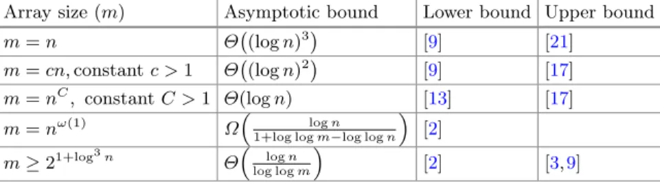
The cost of an algorithm is the maximum over all hostile sequences of the cost of the algorithm on the sequence. We write χn(m, r) for the value of the game, which is the minimum cost of an algorithm.

2 Deterministic Algorithms with Arbitrary Universe

9] showed an amortized lower bound of Ω(log2n) that matched the upper bound in the initial paper of [17]. This lower bound built on previous work by Dietz and Zhang ([12,15], also available in Zhang's PhD thesis [21]) that proved the same lower bound for a limited class of algorithms, called smooth algorithms.

3 The Role of the Universe Size

4 Randomized Online Labeling

Voorlopige versie: Proceedings of the Fourty-Fourth Annual ACM Symposium on Theory of Computing, STOC 2012, pp. In: Proceedings of the Nineteenth Annual ACM Symposium on Theory of Computing, STOC 1987, pp.

Maintaining Chordal Graphs

Dynamically: Improved Upper and Lower Bounds

1 Introduction

Previous Work

10], who gave Ω(logn/log logn) amortized query and update time for fully dynamic connectivity in a sizeO(logn) cell probe model. 9] gave an Ω(logn/log logn) amortized lower bound on the update and query operation for fully dynamic recognition of regular interval graphs with word size O(logn).

Our Results

In this paper we give a formal proof of the Ω(logn) lower bound which also holds for some other subclasses of chord graphs. Finally, we give the first non-trivial lower bound for the fully dynamic maintenance of chord graphs.

Organization of the Paper

The only non-trivial algorithms for problems such as minimal coloring, maximal independent set, minimal clique covering in chord graphs are known via PEO [8]. Thus, our conversion from clique tree to PEO means that all Ibarra results that took O(n) query and update time or more can now be translated directly to PEO and thus all these problems in chordal graphs can also be resolved more efficiently.

2 Decremental Algorithms Using Clique Tree

Structure with a Worst Case Update Time

Update the sorted lists at each of the new nodes formed in the clique tree. Maintaining a counter and pointers for each edge and vertex of the clique tree takes a total time of O(nk2).

Amortized Analysis

If this was the case before, then the new charge atYnbr is at most its old charge plusd+d2 (since the charge atY by induction hypothesis was at most d2 and its degree is at most d). According to the induction hypothesis, the old charge at Ynbr is at most d2nbr, and its new charge is d+dnbr.

3 Dynamic Maintenance of Perfect Elimination Ordering

Decremental Algorithm

So the new charge atYnbr is the old charge in that node plus the charge atY plusd. So the total charge on the existing nodes at any time is at most 4n2 since the sum of the degrees is at most 2n.

Fully Dynamic Maintenance of PEO

Since the bandc are already in line, they were visited earlier in the transition. During traversal, each node is pushed onto the stack only once and popped once.

4 Lower Bound

If it is, then we declare that u and v are in different components of the forest, otherwise they are in the same component. If fu and v are in the same component, then the path in the component between u and wave together with the edges {u, s}, {s, t} and {t, v} forms a chordless cycle.

5 Conclusions

ACM 30(3), 514–550 (1983)

Gavril, F.: Algorithms for minimum coloring, maximum clique, minimum coverage by cliques, and maximum independent set of a chord graph. Mezzini, M., Moscarini, M.: Simple algorithms for minimal triangulation of a graph and backward selection of a decomposable markov network.

Distributed Symmetry-Breaking Algorithms for Congested Cliques

The Congested Clique Model and Problems

Since the publication of the result of [16], many additional problems in the Congested Clique environment have been studied [4–7,11]. Another symmetry-breaking problem studied in the Congested Clique is Maximal Independent Set (henceforth, MIS).

Our Results and Techniques

Thus, our results show that any computable problem can be solved in the congested clique in O(a) rounds deterministically. Distributed Symmetry-Breaking Algorithms for Congested Cliques 45 we obtain an MIS in O(√ . a) time in the congested clique.

Related Work

2 Preliminaries

Definitions

3 Forest-Decomposition-CC

Thus, each vertex can deduce its cluster index H within O(loga) rounds from the start of the algorithm. The last step of the algorithm is to divide the set of edges of the graph into forests as follows: each vertex is responsible for its outgoing edges and assigns each outgoing edge a unique label from the set {1,2,.

In the Arb-Linial procedure each vertex takes into account only the colors of its parents in the forests F1, F2,. The Arb-Coloring-CC procedure computes a proper O(a2) coloring in compressed clique rounds in O(loga+ log∗n).

Given an O(a)-forest decomposition of G, the procedure computes a proper coloring ϕ of the graph using O(a2) colors in O(log∗n) running time. Since the procedure requires each vertex to send only its current color to its neighbors (which is of size O(logn)), the Arb-Linial Procedure can be called as is on the compressed clique.

For graphs G with a(G) = a and a parameter,q=aε, for an arbitrarily small positive constant ε, Procedure Forest-Decomposition-CC splits the edge set of G into A=O(a1+ε)oriented forests iO(1 )rounds in congested cliques. For graphs G with a(G) = a and with a parameter q = aε, for a positive constant ε, Arb-Coloring-CC computes O(a(2+ε)) coloring in O(log∗n) time in congested cliques.

The Clever Shopper Problem

In this work, we investigate the case where a customer wants to buy books in stores with free shipping; In addition, each store offers a discount when purchases exceed a certain threshold (discounts and thresholds are specific to each store). The function D that maps each trade s to the pair (ds, ts) is called the discount function.

2 Hardness Results

Note that the number of stores visited corresponds exactly to the total discount received (ie to parameterize the reduction). We now prove the non-existence of polynomial kernels (under standard complexity assumptions) for Clever Shopper parameterized by the number of books.

3 Positive Results

If we add up all these stores, the total price paid for the books in B∗ is the least. We propose the following dynamic programming algorithm that generalizes the classical pseudo-polynomial partition algorithm.

4 Approximations

Max-Discount Clever Shopper is APX-hard even if each store sells at most 3 books and each book is available in at most 2 stores. Note that for each store S, the amount spent is at least ts, so the total discount obtained by this algorithm is D≥.

5 Conclusion

Our approximation algorithm proceeds as follows: start with a set of selected stores S =∅, a set of available booksB =Band sort the stores by decreasing value of ofds. For such a solution, let D∗ be its total discount, S∗ be the set of stores where purchases reach the threshold, and for any s∈S∗, let Bs∗ be the (nonempty) set of books purchased at stores.

A Tight Lower Bound for Steiner Orientation

Hassin and Megiddo [8] showed that Steiner orientation is polynomial time solvable if the input graphG is completely undirected, i.e. has no directed edges. Is Steiner Orientation FPT on planar graphs, or can we get an improved running time, like f(k) nO(√k).

2 The Reduction

Construction

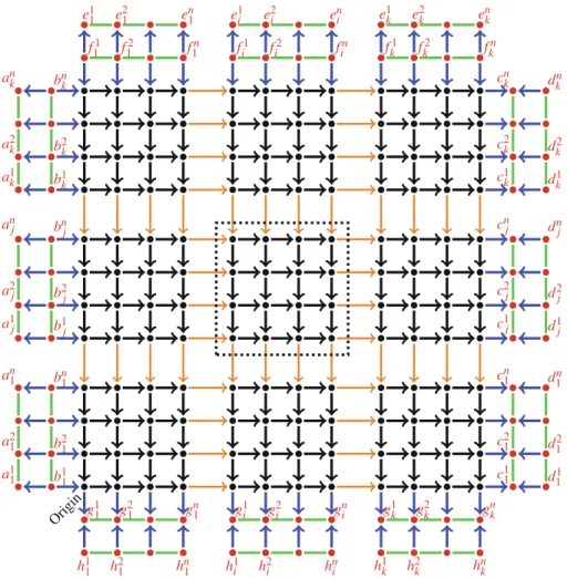
Each row of Gi,j is horizontal and the number of the row increases as we go vertically upwards. Similarly, each column of Gi,j is vertical and the number of the column increases as we go horizontally to the right.

G RID T ILING has a Solution ⇒ S TEINER O RIENTATION

Note that the orientation of G, which orients all dashed edges to the right, i.e. LB→TR, contains each of the horizontal canonical paths defined above. Note that the orientation of G, which orients all dashed edges to the left, i.e. LB←T R, contains each of the vertical canonical paths defined above.

S TEINER O RIENTATION has a Solution ⇒ G RID T ILING

By Lemma2, we know that the paths satisfying the terminal pairs (bni, a1i) and (b1i, ani) cannot contain yellow edges. By Lemma6, we know that the orientation G∗ must contain the horizontal canonical pathQλjj (to satisfy the pair (b1j, cnj)) and also the vertical canonical path Piδi (to satisfy the pair (fin, gi1)).

Can We Create Large k -Cores by Adding Few Edges?

It is also NP-hard to approximate the optimal kernel size within a factor of O(n1−)1 for every >0. Edgek-Kernel (EKC) problem: In this paper we consider an alternative way to maximize the size of the kernel k.

2 Classical Complexity: Polytime Algorithms and NP-hardness

If k = 2n and p = 4n, then the number of vertices that must be anchored to obtain anchored k-kernel of size p is bv = 2n. But to get a pure k-kernel of size p, it is enough to add the n edges of the perfect match that were removed from G2.

3 Parameterized Complexity: W[1]-Hardness and FPT Algorithms

• Leaf Node
• Forget Node
• Introduce Node
• Join Node

Also, let Vt denote the union of nodes in all bags of the nodes in the subtree of T rooted att, i.e. Vt=∪t∈TtBt. If it isn't, then we can call the child with almost exactly the same values; if it is in the thek core, then we guess at the exact connections that the forgotten node will have to other vertices in the bag.

4 Conclusions and Future Directions

Chwe, M.: Structure and strategy in collective action 1. Chwe, M.: Communication and coordination in social networks. Dezs˝o, Z., Barab´asi, A.: Blocking viruses in scale-free networks. In: Proceedings of the 9th WebKDD and 1st SNA-KDD 2007 Workshop on Web Mining and Social Network Analysis, pp.

Periodicity in Data Streams with Wildcards

Our Contributions

The challenge of determining periodicity in the presence of wildcards can first be addressed by working toward an understanding of specific structural properties of wildcard strings. We show in Lemma2 that the number of possible assignments to the wildcards over all periods is

Related Work

Finally, in the full version of the article in [EGSZ18], we note several results in the related problem of determining the distance to p-periodicity.

Preliminaries

At first glance you might think that assigning the character 'b' to the wildcard character in the prefix S[1, n−1] and an 'a' in the suffix S[2, n] would separate the prefix and the suffix will make identical. In addition, this encoding supports string concatenation and can be performed in the streaming setting.

2 Our Approach

Whereas exact and k-periodicity can be verified by comparing the number of prefix-suffix mismatches of length n−p, wildcard periodicity is sensitive to the correct assignments of the wildcards. We solve this challenge by noting W, the location of the wildcards in the first pass.

3 Two-Pass Algorithm to Compute Wildcard-Periods

Computing Small Wildcard-Periods

We can find the assignments of the wildcards in the second round by looking at the characters in a few places, which we determine viaW. Output: A concise representation of all candidate wildcard periods and the location of the wildcards.

Verifying Candidates

The second obstacle is dealing with wildcards when calculating the fingerprints of S[1, n−t] and S[t+ 1, n]. We can then verify whether or not pi is a wildcard period of S if the mapping of the wildcard characters with respect to topi is also known.

Computing Large Wildcard-Periods

We describe the first review in full in the full version of the paper in [EGSZ18]. The running time of the algorithm is dominated by the time spent logging parallel copies of the k-mismatch algorithm in the first pass.

4 Lower Bounds

Implied from Theorem 3 from [EJS10] and Theorem 16 from [EGSZ17]). Given a string S with at most k wildcard characters, any

Bob then proceeds to run the algorithm on x◦x◦x to determine the wildcard period of the string S(x, y) =y◦x◦x◦x. In: Proceedings of the Forty-Fifth Annual ACM Symposium on Theory of Computing, p.

Maximum Colorful Cycles in Vertex-Colored Graphs

However, in our paper we exploit these algorithms to construct a Hamiltonian cycle for a given set of candidate vertices in a maximal colorful cycle. The problems of the tropical subgraph and the maximal colorful subgraphs in vertex-colored graphs have been studied recently.

2 Hardness Results for MCCP

Now from a truth assignment B with all fulfilled clauses it is possible to obtain a cycle with all colors as follows. Conversely, from a cycle K containing all colors Gc, we obtain the following assignment with all satisfied clauses.

3 An Algorithm for MCCP in Threshold Graphs

Algorithm for Threshold Graphs

Based on the structural properties of maximal colorful cycles according to different cases, we derive the following algorithm to find a maximal colorful cycle. The algorithm makes use of the algorithm that computes a maximal colorful matching [5] and the algorithm that computes a Hamiltonian cycle in threshold graphs [14].

4 An Algorithm for Bipartite Chain Graphs

Grammar-Based Compression of Unranked Trees

While a peak day can be transformed in linear time into an equivalent FSLP with a constant multiplicative inflation (Theorem6), the reverse transformation (from an FSLP to a peak day) takes timeO(σ n) and involves a multiplicative magnification of size O(σ) where σ is the number of node labels of the tree (Proposition7). Theorem 13 also holds if the trees t1 and t2 are given by topdags or TSLPs for the fcns encodings, since these formalisms can be efficiently converted to FSLPs.

2 Straight-Line Programs over Algebras

Grammar-based compression of unordered trees 121 It will be convenient to allow for the right-hand side ρ(A) algebraic expressions over A, where the variables of V can appear as atomic expressions. We define the magnitude |P| of an SLP P as the total number of occurrences of operations f1,.

3 Forest Algebras and Forest Straight-Line Programs

Forest outline programs. Aforest straight line programmerΣ, FSLP for short, is a valid straight line program over the algebra FA(Σ) such that F∈ F0(Σ). Grammar-Based Compression of Unsorted Trees 123 FSLPs generalize tree-level programs (TSLPs for short) previously used to compress sorted trees, see e.g.

4 Cluster Algebras and Top Dags

5 Relative Succinctness

From a given FSLPF one can construct in linear time a FSLP F in normal form such that F=F and|F| ∈O(|F|). Given a tree t of size n with σ many node labels, one can in linear time construct an FSLP for t (or a TSLP for fcns(t)) of size O(n/logσn)∩O(d ·logn) construct, the size of the minimal day is often the value.

6 Testing Equality Modulo Associativity and Commutativity

Associative Symbols

Commutative Symbols

From a given FSLPF = (V, S, ρ) in normal form, we can in polynomial time construct a FSLPF= (V, S, ρ) in strong normal form with F= F. The main idea is that the strong normal form ensures that in right side of forma(DxE) with en∈ Cone can move the parameterx to the last position (see point 3 above) since only trees are larger than all trees produced from.

7 Future Work

By Lemma18, we can calculate in polynomial time a total sequence

Complement for Two-Way Alternating Automata

However, since 2AFAs do not have the resources to count steps performed, the trivial construction does not work for 2AFAs with infinite loops. This complementary simulation does not require the elimination of infinite loops in the original alternating machine, but the complemented machine itself comes to infinite loops along some computational paths.

2 Two-Way Alternating Automata, Preliminaries

For a given input, consider the tree of all computational paths starting at the initial configuration q0,0. The given entry is accepted if the tree rooted in the initial configuration accepts.

3 Deterministic Machines with Linear Space

The read/write component C in the cell will be used to store the navigation data during the depth search. This activates a backup routine against the direction of the edge connecting the current parentr, k−d to q, k , reachingr, k−d in the accept,0 state. c) A comes to the cell of the work tape corresponding toq, k from one of his sons, in statuses reject,0.

4 Two-Way Alternating Automata, Complemented

Furthermore, A does not visit any cell along the work bar more than O(n2) times during the entire computation. Furthermore, A must move the head from ST in the -d direction, since the path connecting S2 to S does not visit the same work tape position in the meantime.

5 Concluding Remarks

Complement of two-way alternating automata 143 Despite Theorem 2, it is still open whether we can transform every n-state 2AFA into a halting 2AFA with a polynomial number of states. The most important is the case ofk= 1, i.e. the cost of complementing a two-way automaton that makes only existential choices with a two-way automaton that makes only universal choices, or vice versa.

Closure Under Reversal of Languages over Infinite Alphabets

Each pebble can serve as the head of the automaton or point to a position in the input word. In Sect.2 we present the definition of wPA and state the separation theorem whose proof, for the case of 2-wPA, is presented in Sect.3.1 In Sect.4 we show how the languages ​​L⊆ and L⊇ are changed into languages ​​whose words does not contain a distinguished punctuation mark.

2 Weak Pebble Automata

That is, the run starts in the initial state s0, with pebble 1 placed at the beginning of the input word. Only pebble 1 can reach a final state and only after it falls down from the right side of the input.

3 Proof of Theorem 1

Since there are 2 equivalence classes modulo 2 and the number of different states in the sequence is limited by |S|, there are two indices j1 and j2,. This is because pebble 1 must arrive at position|u| in the same state in the Aonwandw runs and these runs depend on the total entries.

4 Removing the Distinguished Separator Symbol $

5 Concluding Remark

Structural Parameterizations of Dominating Set Variants

Motivation

Note that there may not be an effective dominating set for a graph (for example, for a 4-cycle). The standard dominating set and most of its variants are NP-hard or W[2]-hard in split graphs [20].

2 Preliminaries and Notations

SET-COVER, parameterized by the size of the universe, does not allow any polynomial kernel, unless NP⊆coNP/poly. CNF-SAT, parameterized by the number of variables, does not allow a polynomial kernel unless NP⊆coNP/poly.

3 Related Work

There is no >0 such that SET COVER can be solved in O∗((2−)n) time, where n is the size of the universe.

4 Dominating Set Variants Parameterized by CVD Size

Upper Bounds

Structural parameterizations of dominant set variants 163 Lemma 2 ().1 Set-Cover with partition can be solved in O∗(2|U|)time. We construct the Set-Cover with Partition instance from the DS disjointcluster instance as discussed above.

Lower Bounds

It is easy to see that a size solution exists in the DS-disjointcluster instance if and only if a size solution exists in the Set-Cover with Partition instance. For each guess S⊆S with|S|=i we now construct the Set-Cover with Partition instance with|U| ≤k−i and solve with running time O∗(2k−i).

5 Dominating Set Variants Parameterized by SVD Size

EDS and IDS Parameterized by SVD Size

If T is a minimal vertex cover of the graph G, then V(G)\T is an independently dominating set in G. From Observation1, we know that the complement of a maximally minimal vertex cover is a minimal independently dominating set.

Improved Algorithm for EDS-SVD

For EDS, because the size of the SVD set is always smaller than the size of the vertex coverage, we have the following corollary to Theorem 8. Because Branching Rule 1, Reduction Rule 1, and Branching Rule 2 do not apply, by the following lemma with which we can choose v arbitrarily.

6 Concluding Remarks

Courcelle, B., Makowsky, J.A., Rotics, U.: Time-solvable linear optimization problems on bounded clique width graphs. Cygan, M., Pilipczuk, M.: Split vertex deletion meets vertex cover: new fixed parameter and exact exponential-time algorithms.

Complexity and Inapproximability Results for Parallel Task Scheduling