Raimund Seidel (Universität des Saarlandes und Schloss Dagstuhl – Leibniz-Zentrum für Informatik) Thomas Schwentick (TU Dortmund). Dieser Band enthält die beigesteuerten Beiträge und Abstracts der eingeladenen Vorträge, die auf der Konferenz gehalten wurden.
List of Reviewers
Siddharth Bhandari
Prahladh Harsha
Tulasimohan Molli
Srikanth Srinivasan
1 Introduction
Furthermore, since all upper bound constructions for OR polynomials are polynomials covering hyperplanes, we not only have that P-degε(ORn) =O. For this class of polynomials, we prove the following (almost) tight result on the error hyperplane ε covering the probability degree OR.
2 Upper bounds on probabilistic degree of OR
A special class of hyperplanes covering polynomials for which Alon, Bar-Noy, Peleg and Linial [1] proved a similar limit is the class of hyperplanes covering polynomials where the linear forms are sums of variables (i.e., Li(¯z) = P .j∈Sizj for some Si ⊆ [n]). Ideally, we would like to extend the lower bound result for polynomials spanning the hyperspace where linear forms are sums of variables to all polynomials.
3 Lower bound on hyperplane covering degree of OR
Proof outline
Then, by the anti-concentration of linear forms over rules (Lemma 3.7), we have that every linear form is 1 with probability at most. We can then show that a combination of the above two arguments will still work if the remaining linear forms have the following nice structure.
Proof of Theorem 3.4
To this end, we first apply Proposition 3.9 in setLoftlinear form to the polynomial P to obtain it. The size of L0 is the number of iterations of the while loop and is thus bounded above by R.
Restricted Parse Trees
The model of study
A related set-depth-∆ formula model was studied by Agrawal, Saha, and Saxena [3], which is a subclass of UPT circuits where the underlying parse trees are extremely regular3. Lagarde, Malod and Perifel [18] extended the techniques of Nisan [20] to give exponential lower bounds for UPT circuits.
Polynomial identity testing
Our results
Polynomial Identity Testing
Structural results
Proof ideas
To establish the depth reduction (Theorem 1.4) we follow the strategy of Valiant, Skyum, Berkowitz and Rackoff [27] and Allender, Jiao, Mahajan and Vinay [4] but make use of the UPT structure (work with different boundary nodes and gate quotients) based on the underlying shape of the parse trees. It was pointed out to us that the key ideas in our proof of depth reduction were used by Arvind and Raja ([5]) for a commutative analogue of UPT circuits.
2 Preliminaries 2.1 Notation
Basic definitions UPT and FewPT circuits
Furthermore, the width of the ABP is directly related to the sample width of the resulting UPT circuit.
Shuffling of a polynomial
Basic lemmas
Canonical UPT circuits, and types of gates
3 Depth reduction for UPT circuits
UPT ⊗-circuits
Furthermore, each coordinate of tuple ([u:w],[w1],[w2]) is all of the same type as we walk over alw∼τ. We need a slightly stronger inductive hypothesis which is that the choice of permutationσ depends only on the shape of the parse trees inC0.
UPT circuits of constant width
The next consequence is immediately from the fact that any circuit of depth and magnitudes can be calculated by a formula of magnitudesO(d) and therefore an ABP of magnitudesO(d).
4 Separating ROABPs and UPT circuits
The polynomial
Let Td denote the complete binary tree of depth (with 2d leaves) and let D= 2d+1−1 refer to the number of nodes in Td. We will say that a coloringγ:Td→Zm is legal if for every nodeu∈T, if the children of outhenγ(u) =γ(v) +γ(w) are modm.
5 Hitting sets for non-commutative models Commutative brethren of non-commutative models
Hitting sets for UPT set-multilinear circuits
Poly-sized hitting sets for constant width UPT circuits
6 FewPT circuits
Preliminaries
Let C be the class of n-variate degree set multilinear polynomials (with respect to toy=y1t · · · tyd) computable by UPT set multilinear circuits with preimage-width-wand-depth r. We further qualify this notation to use Σk-UPT(w) to denote the class of circuits that is the sum of k preimage-width UPT circuits.
Notation
Suppose wt : y → Mr is a BIWA for the class of polynomials computed simultaneously by UPT-SML circuits with sample width at most w2O(k). There is an explicit hit set Hd,n,s,k of at most size(s2knd)O(logd) for the class of n-variable degree dhomogeneous non-commutative polynomials inFhx1,.
7 Open problems
Then the polynomial f(y+twt)∈F(t)[y] has a monomial with a nonzero coefficient that depends on at most 2O(k)logw variables iny. Preliminary version of the 6th International Symposium on the Mathematical Foundations of Computer Science (MFCS 1981).
A Relative computational power of restricted parse tree models
Constant width models
- ABPs vs constant width UPT circuits
We can obtain a strict separation between constant width ABPs and constant width UPT circuits using the proof of Theorem 1.5. A more interesting comparison is that of ABPs of unbounded (poly(n)) width and constant width UPT circuits, which we now discuss.
Rank, Degree, and Number of Generators
Arvind
Abhranil Chatterjee
Rajit Datta
Partha Mukhopadhyay
The permanent computation of an n×n matrix over any field F can be cast in terms of the univariate ideal membership. This naturally raises the question of whether ideal one-sided membership is in conNP when each generating polynomial has distinct roots.
2 Preliminaries
The distinct roots case discussed in Theorem 8 is in sharp contrast to the complexity of testing membership of PA(X) in the ideal hx21,. Note that in general rootsαi∈Cand in the standard Turing Machine model the NP machine cannot guess the roots directly with only limited precision.
3 Ideal Membership for Low Rank Polynomials
Proof of Theorem 3
First, assume that field arithmetic over F can be implemented using polynomial bits and L is the upper bound on the bit size for each coefficient inf, p1,. We will show that the circuit we use in the next recursive step has bit size coefficients at most L˜+poly(n, d, L).
Vertex Cover Detection in Low Rank Graphs
4 Parameterized Complexity of Univariate Ideals
Parameterized by the Degree of the Polynomial
- Proof of Theorem 5
There exists an efficient randomized algorithm that constructs with constant probability a homogeneous degree k-diagonal circuit Do of top fan-inO∗(4.08k), which computes a polynomial weakly equivalent to the polynomial g (defined before Lemma 23). By a direct calculation one can obtain a diagonal circuitD of top fan-in O∗(4.08k) which is weakly equivalent to the polynomialSm,k.
Parameterized by Number of Generators
- Proof of Theorem 7
For each columnj, think of the consecutive 2 lognbits as the binary extension of a single entry, call it N and set A[i][j] to N. When t is odd, the bit is 1 and so there must be a 1 in the corresponding bit of (Pn . j=1aijt·zj).
5 Non-deterministic Algorithm for Univariate Ideal Membership
Proof of Theorem 8
It is important to note that the parameterM can be efficiently precomputed from the input parameters. Now we show how to verify that the guessed point ~α˜ is a good approximation of the roots for the univariate polynomials.
Parosh Aziz Abdulla
Mohamed Faouzi Atig
Shankara Narayanan Krishna
Shaan Vaidya
The control mode accessibility problem was found to be solvable with an EXPSPACE lower bound under this model. Furthermore, the control state availability for the model presented in [7] is undecidable, while it is decidable for our model.
3 Multiset Timed Automata
Given a certain number of locations s=(s1, . . sN) of anN-MTAM, the control state reachability problem asks whether, given the initial configuration c0 of M, there is a run that has a configuration c=( q, m) reached. ) so that qi= (si, νi) for somem, and for someνi, for all 1≤i≤N. Given a given tuple of locationss=(s1, . . sN) of an N-MTAM, the configuration reachability problem asks whether, given the initial configuration c0 of M, there is a run that has a configuration c=(q,m ) reaches such that m=.
4 Control State Reachability
Now we are ready to propose a 1-safe timed Petri net (with reading arcs) whose coverage problem is equivalent to the control mode availability problem for the given N-MTA. The control mode availability of M thus reduces to the coverage of the constructed 1-safe timed Petri net with reading arcs.
5 Configuration Reachability
The number of pending tasks of typea (resp. b) corresponds to the value of counter c1 (resp. c2). A detailed discussion with proofs of the lemmas can be found in the extended version of the paper [1].
6 Conclusion
Vaandrager, editors, Formal Modeling and Analysis of Timed Systems, 7th International Conference, FORMATS 2009, Budapest, Hungary, September. InTools and Algorithms for the Construction and Analysis of Systems - 22nd International Conference, TACAS, volume 9636 of Lecture Notes in Computer Science, pages 680–697.
Chris Köcher
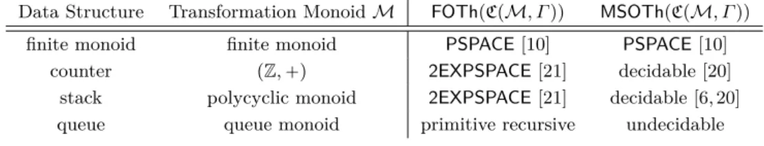
Concretely, we will see that this graph's first-order theory is determinable by giving a primitive recursive (but non-elementary) algorithm that combines two well-known methods from model theory in a (at least for the authors) new way: the method of Ferrante and Rackoff [8]. The type of a structure is the collection of all first-order sentencesϕ of quantifier rank at most such that G|ùϕ.
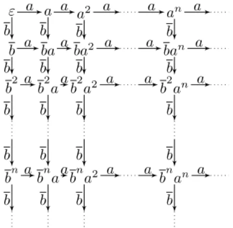
3 Queue Monoid and its Cayley-Graph Definition of the Monoid
We then give some general properties and some special features of the Cayley graph of the queuing monoid. The concrete form of the Cayley graph of the monoid strongly depends on the chosen set of generators.
4 Combinatorics on Words
A complete boundary decomposition of uPA˚ is therefore the sequence of all boundaries ofu, ordered by word length. Thus, it is easy to observe that each word uPA˚ has exactly one complete boundary decomposition.
5 Decidability of the FO-Theory
However, we cannot guarantee that every element in close proximity to a given element pc can be associated with a position in the skeleton of p, because small changes in the reads and writes can dramatically change the boundary decomposition. There are two possible types of configurations for pi and pj, so that they can be connected by an edge.

6 Conclusion and Open Problems
We develop a method to analyze the complexity of uniform tree automata presentations, allowing us to provide upper bounds on the running time of the automata-based model checking algorithm for the presented class. FO model checking is FPT on the class of all finite abelian groups succinctly encoded by the orders of the direct product factors and can be performed in exp4(poly(|ϕ|))·log|G|.
3 Model Checking Revisited
We begin with a detailed description of the model checking algorithm on structures given by adviceα from a uniform tree autopresenter. Note that for the runtime analysis in the next section, it is crucial that we construct only the reachable states of the product automaton.
4 A Presentation Aware Runtime Analysis
Let be a uniform tree automata representation of class C and let (Emr)r,m∈N be an EF-congruence with respect to c. Let C be a uniformly tree-like automatic representation of a class of τ-structures and let I be a parameterized τ-v-σ-interpretation of breadth that for each A∈ C interprets the structure I(A).
5 FPT Model Checking With Elementary Parameter Dependence
Boolean Algebras
It is known that the theory of all finite Boolean algebras is complete for the complexity class S. If we could perform model checking in timeO(2poly|ϕ|·log|B|), then we could solve the theory of finite Boolean algebras in time O.
Finite Groups
Then I(N,+)(n) ∼= Zn for all n ∈ N and therefore Id is a uniform representation of the class of all finite cyclic groups. Furthermore, (Id)× is a uniform representation of the class of all finite abelian groups and Theorem 4.6 tells us that it is a (g(r+m)r)g(r+m) ∈exp4(poly(|ϕ|) ) bounded EF congruence.
Graphs of bounded Tree-Depth and MSO Model Checking
First-order model checking is FPT on the class of all finite groups with bounded non-abelian decomposition width. In Michael Kaminski and Simone Martini, editors, Computer Science Logic, number 5213 in Lecture Notes in Computer Science, pages 431–445.
A Proofs Omitted from Section 4
In fact, we prove an extended claim, namely that the procedure computes the automaton Aϕ at the given time and Aϕ has the property δ∗A. Consequently, the number of available states in the aforementioned power set automaton is bounded by f(m+r).
B Proofs Omitted from Section 5
Then the class C of all power structures of tree depth graphs maximally sets its uniform tree automatically. Otherwise, t could be the slope of a tree T with depth at mosth+ 1, but there is a note v∈Tof depthi with v∈PiTandi+ 1≥j.
Theorem
Elazar Goldenberg
- Our Results
- A General Direct Product Theorem
- Sliding Window Domain
- Technical Contribution: Proof Overview of Theorem 2
- Related Work
- Organization of the Paper
We then show our key technical result that coordinated expansion implies direct product testing (for a given range of parameters). Note that |A| =n and yet we show that it allows a direct product theorem (see Theorem 9 for a simple proof).
3 Direct Product Testing: The Setting
Furthermore, the above setting of direct product testing can be generalized to the case where V is a multiset P([n]), and the results in this paper still hold. The above remark also applies to the case of studying test graphs that are not regular in degree, which are not discussed in this article.
4 Direct Product Testing: Coordinate Expansion
With probability (1−2c)β testT0 selects S∈B(c,1−c) and we would like to analyze the rejection probability conditional on this. Note that under the assumption that T0 chooses i0 =i and S ∈B˜i , sets S with few conflicting coordinates are more likely to be chosen than those with many.
5 Sliding Window Domain
In Appendix B, we discuss the test plot J(n, k, k/2) and show the direct product theorem when close ton/2. This is because for gap and hardness applications it is desirable that the direct product domain also have distance amplification (defined below), and high-dimensional expanders have distance amplification while the sliding window domain does not.
A Missing Proofs
Thus, the construction of the sliding window domain provides a conceptual explanation for why we need high-dimensional expansions: we can obtain direct product testing of simple constructions such as the sliding window domain and we can obtain distance amplification of known constructions of vertex expanders (see Appendix D) ; but to obtain both simultaneously, [6] needs high-dimensional expansions. A Subconstant Error Probability Low-Grade Test, and a Subconstant Error Probability PCP Characterization of NP.
B Application of Theorem 8: Ω(n)-slice of the Hypercube
C Simple Applications of Lemma 10
As a consequence, we get that we test the direct product encoding when domainV is equal. Also for everyS ∈V and everyi∈S the probability of a uniformly random neighbor S0 of S in Gcontainsi is 1/2.
D Linear Sized Domains having Distance Amplification
Schemes Storing Three Elements
Deepanjan Kesh
The Bitprobe Model
The Problem Statement
2 Two Bitprobe Schemes
The Decision Tree
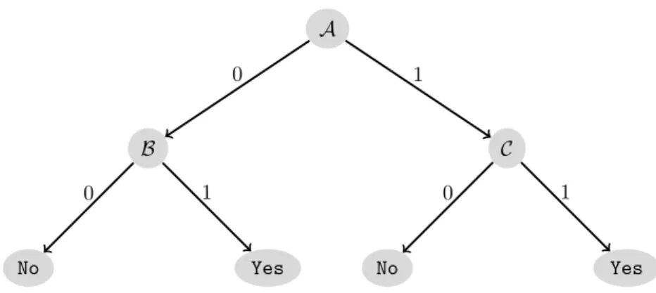
Given a subset of universeU, the storage schema places the parts of these tables in such a way that the query schema correctly answers membership queries. The query schema description can be represented in the form of a tree, shown in Figure 1, and is known as a decision tree.
Blocks
The arrangement and purpose of these three tables will be more apparent from the query schema discussed below. Depending on whether the bit stored in the location is a 0 or a 1, the second bit probe is performed on table B or C.
Sets
3 Clean and Dirty Sets
We will prove that the elements of this block will necessarily belong to different sets in tableau C. Thus, we can conclude that the elements of block a must belong to different sets v.
4 Mass of a set
We can do the same exercise for tableC and count the total number of elements in all the blocks responsible for creating dirty sets in tableC. J It is interesting to note that the total mass of one of the tables BandC is minimized when all the blocks in tableA are of equal size.
5 Bad Elements
- Property of a bad element
- Universe of X
- Bounded Sets of Table C
- Large Sets of Table B
Considering the fact that x2 is a member of the subsetS, the bit corresponding to the setZ in tableB must be set to 1 (Figure 3). The total mass of the large sets of table B is less than or equal to the total mass of the bounded sets of table C.
6 The Lower Bound
If the total number of elements is 2m, then Lemma 10 tells us that the total mass of all the sets of tableB or tableC is at least. In the case that all the sets of table C are bounded, then the total mass of all bounded sets is at most.
7 Conclusion
Siddhesh Chaubal
Anna Gál
Previous Constructions with Quadratic Separation
All previous constructions that achieve a quadratic separation between sensitivity and block sensitivity - with the exception of Chakraborty's functions [7] - were based on the following. The quadratic separations of are based on using this lemma and considering functions of the formf =ORn◦g for appropriately chosen inner functionsg.
3 New Building Blocks for Quadratic Separation
- A General Framework Based on Certificates
- Using Finite Field Multiplication
- Using Polynomial Multiplication
- s 0 (g poly ) = 2
- bs 0 (g poly ) = m
- bs 1 (g poly ) = m + 1
We first note that the set of subassignmentsAlso forms a set of 1-certificates forgC such that each 1-input matches exactly one subassignment fromC. This follows from property (a) of a good set of partial assignments, since: for any 0-inputx, there is at most one certificateci∈C which is at a distance 1 from it.
4 Additional Properties of Function Composition
So if xi = 0, we choose as yi a 0-input ofg on which its 0-block sensitivity is achieved, and similarly, ifxi = 1, we choose asyi a 1-input ofgon on which its 1-block sensitivity is achieved become By comparing the statement of Lemma 35 with Lemma 11 of Tal [17], we notice that in the context of 0-block sensitivity and 1-block sensitivity it is enough to require an additional condition for the outer function .
This gives at least bs0(f)·min{bs0(g), bs1(g)} discrete sensible blocks forf◦g in the input, and the first equation follows. This theorem allows us to use different compositions of our new building blocks and some of the inner functions of the previous constructions to obtain other functions with 0-block sensitivity and 1-block sensitivity quadratically greater than sensitivity.
Well-Quasi-Ordered
Kazuyuki Asada
Naoki Kobayashi
The (ordered) alphabet Σ is a mapping from a bounded set of constants (representing the tree constructors) to the set of natural numbers called arities. For a closed landλ→-termt, L(t) is a monotonic group{π}; we write T(t) for such π and often call it the tree.
Some quasi-orderings and their logical relation extension
Each quasi-ordering for higher-order terms used in this article is a logical relation extension (of some basic quasi-ordering). The following is the quasi-ordering used in the theorems in this article.
3 Numeric Pumping Lemma for Higher-order Tree Languages
4 Numeric Version of Order-3 Kruskal’s Tree Theorem
Main theorem
For any alphabet Σ, any a∈Σ, and any order-2 type environmentΓ (i.e., a type environment whose codomain consists of types of order up to 2), the quasi-orders #,Σ,aΓ,o onΛ∅Γ, o is a wqo. For Theorem 14, it is sufficient that #,Σ,aκ on ΛΣκ is a wqo for everya∈Σ andκ with order(κ)≤3, because#,Σκ = ∩a∈Σ(#,Σ,aκ ) and well-quasi -orders are closed under finite crossing.
Transformation from order-3 terms to order-2 terms
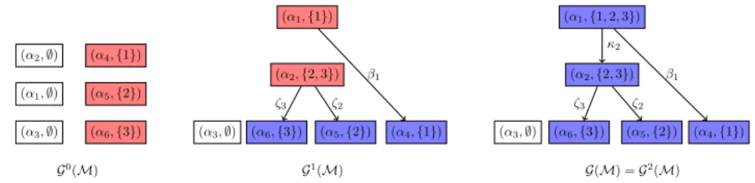
The output of the transformation consists of three parts, separated by semicolons: a (possibly empty) sequencev1,. The proof of the above lemma is given in the full version, where we use Lemma 17 and the substitution lemmas in the external variables.
N on order-2 terms is a wqo
Note that f0 0 is a Φ-normal form; the first rule is not applicable since f0 06NΦ0 after the discussion in Example 24. The following lemma ensures that any polynomial of order 2 can be transformed into at least one equivalent (Φi)i-normal form.
5 Conclusion
According to Kruskal's tree theorem, he,Σo N∪Γ on PNΓ,o is a wqo, and hence the suborderinghe,Σo N∪Γ on the subset.
David Baelde
Anthony Lick
Sylvain Schmitz
While linear-time logic is less expressive than FO(<), first-order logic over linear orders with unary predicates, it nevertheless has nice characterizations as it captures its two-variable fragment FO2(<) instead [ 13]. This is satisfactory since KtL`.3 is simply obtained from Kt4.3 – the tensed logic of arbitrary linear time streams – by adding a good basis to the left, i.e.
2 Tense Logic over Ordinals 2.1 Syntax
Ordinal Semantics
Moreover, our proof system is easily shown in Section 4 to also handle more exact validation problems over all well-grounded linear time courses. But more importantly, they give a system of proofs for FO2(<) over ordinals, which would be challenging to construct directly, because the eigenvariables cannot be treated in the usual way.
3 Hypersequents with Clusters
- Annotated Hypersequents with Clusters
- Semantics
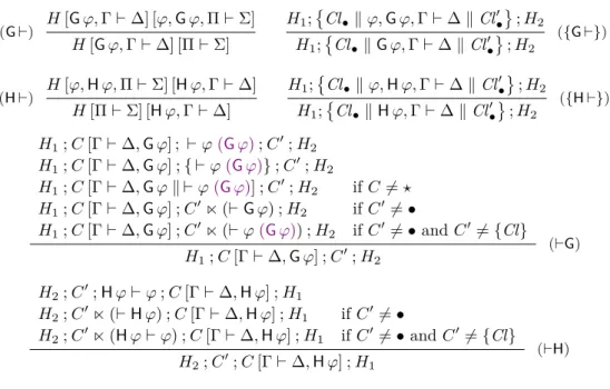
- Proof System
- Soundness
- Completeness and Complexity
Considering the rule example with the countermodel (M, µ) of the premise H, we construct the countermodel (M, µ0) of the conclusion H0. This can be seen, for example, from the first premise of the third application of the rule (`H) in Figure 6.
4 Logic on Given Ordinals
If ϕ holds in all worlds of all structures of the form (α, V) for some V, the hypersequences are valid and can therefore be proved in HKtL`.3 by (ordα).
5 Related Work and Conclusion
These were inspired by the small model feature of Kt4.3[26], and it is notable that we were able to put them to work in the significantly richer setting of KtL`.3; it is the main technical contribution of this article. This shift in perspective, together with the addition of rule ((G)), makes it possible to get rid of the somewhat troublesome use of different semantics for the soundness and completeness of HKt4.3.
A Axiomatisation
B Detailed Proofs
If C0;H2 is not empty, let it be the first position of the concluding hypersequence, which is in C0. If γ is the ordinal of the successor, then (M, µ0) is the countermodel of the first premise simply because the predecessor γ cancels ϕ and the note is obeyed; it holds both by design.
Recognizable
Denis Kuperberg
Related Works
In [1], examples of Büchi and coBüchi GFG automata were given which do not contain any equivalent deterministic subautomata. In [15], it is shown that for co-Büchi automata (and all higher parity conditions), GFG automata can be exponentially more compact than deterministic ones.
2 Definitions
Automata
Typeness properties of GFG automata are captured in [2], as well as the complexity of switching between different acceptance conditions. In [14], the model of GFG automata is generalized to the idea of the width of a non-deterministic automaton, GFG automata corresponding to width 1 , and an incremental algorithm is given to build GFG automata from non- deterministic automata.
Games
- Winning Conditions