Persistence and Determinants of Firm Profit in Emerging Markets

(1)

CESIS

Electronic Working Paper Series

Paper No. 151

Persistence and Determinants of Firm Profit in Emerging Markets

Andreas Stephan

(Jönköping International Business School, DIW Berlin, CISEG, CESIS)

Andriy Tsapin

(Europa-Universität Viadrina)

October 2008

(2)

Persistence and Determinants of Firm Prot in Emerging Markets

Andreas Stephan

^∗

, Andriy Tsapin

^†

October 15, 2008

Abstract

The paper studies the persistence of prot and its determinants in emerging markets. We apply Markov chain analysis, dynamic panel GMM estimation, and quantile regression techniques to a panel of approximately 3,000 Ukrainian companies.

The empirical results show a moderate level of prot persistence, as well as a relatively low speed of adjustment to the steady-state prot level, thus providing no support for the hypothesis that there is a lower persistence of prots in emerging markets due to more intense competition. Regarding the determinants of rm prot in an emerging market economy, the ndings from alternative methods re- veal that ownership structure and regional location of the rm have a signicant impact.

Keywords: Prot, Persistence, Convergence, Markov chain analysis, Ukraine.

JEL Classication Numbers: G32, G30

∗Jönköping International Business School, DIW Berlin, CISEG and Centre of Excellence for Science and Innovation Studies (CESIS), Royal Institute of Technology, Stockholm.

†Corresponding author. European University Viadrina, Frankfurt (Oder), Germany. E-mail address:

atsapin@euv-o.de.

The authors thank Oleksandr Talavera and Daniel Wiberg for their helpful comments on a previous

(3)

1 Introduction

A basic premise of economic theory is that company prot rates should converge to equality in competitive markets. Empirical studies, however, frequently nd that dierences in prots across rms tend to persist over time. Moreover, there is considerable variation across countries as to the speed with which rm prots adjust (or reach) their permanent values (e.g., Cubbin and Geroski 1987, Waring 1996, Glen and Singh 2004).

These dierences could be due to the varying strength of anti-trust policies and country- specic regulatory systems (Geroski and Jacquemin 1988). One of the main conclusions of the literature has been that rivalry alone does not erase persistent asymmetries among rms.

The issue of the persistence of prot has been intensively investigated for advanced market economies, but the evidence for emerging market economies is rather scarce, probably due to lack of appropriate micro data. A study of emerging markets by Glen and Singh (2003) nds that both short- and long-term persistence of protability are lower in these markets compared to advanced markets. The authors conclude from this nding that competition intensity is higher in emerging due to: (i) lower sunk cost to enter markets, (ii) faster growth rates of rms, (iii) weaker role of governmental regulations, and (iv) the existence of many large business groups.

The aim of our study is to present further evidence on the persistence of prot in emerging markets by employing alternative methods in the empirical analysis. In addition, we study the determinants of rm prot as it provides further interesting insights into the dierences between emerging and advanced market economies. For example, the process of ownership structure establishment in transition economies is fundamentally dierent from that observed in more advanced economies.¹ In emerging economies, strong ownership concentration negatively aects rm performance as do underdeveloped capital markets.² Accordingly, we provide evidence on the determinants of prot related to the specicities of transition economies. In particular, we study the

1See Pivovarsky (2001).

2Poorly functioning credit markets may constrain the expansion of companies (Tybout 2000).

(4)

role of rms' intangible assets, companies' ownership structure, and rm location play in regard to protability.

In the empirical analysis we employ three dierent, but complementary, methods.

First, in a novel approach, we use Markov chain analysis for studying the persistence of prot because persistence can be dened as the probability of remaining in the initial prot class. The Markov chain approach has the further advantage of allowing us to investigate the mobility of rms across dierent prot classes, i.e., their likelihood of switching prot classes. Second, we apply dynamic panel data analysis to assess the speed of adjustment of rm prot. Finally, to study the determinants of prots in emerging markets we use quantile regression techniques, which provide more valuable insights in this context than does the standard linear regression model. The rest of the paper is organized as follows. Section 2 provides a short literature review. Section 3 describes our data. In Section 4, the empirical analysis is performed using the Markov chain approach, dynamic panel data estimation, and quantile regressions. Section 5 sets out our conclusions.

2 Literature Review

Numerous studies present evidence that the average rm's prot comprises both permanent and short-run components, and that short-run shocks converge over time (see, e.g., Mueller 1986). Earlier studies have estimated one rate of persistence of prof- itability for all rms. To avoid misleading results, Waring (1996) proposes considering a rm's protability as a combination of a competitive return component, an industry rent component common to all rms in the industry, and a rm-specic rent component.³

The traditional structure-conduct-performance paradigm is challenged by more recent research that distinguishes between industry- and rm-specic eects.⁴ McGahan (1999) nds that both rm and industry inuences are important, stating that (i) organi-

3Mueller (1977) argues that rm prot is comprised of a competitive return, a permanent rent component, and a transitory rent component.

4The structure-conduct-performance paradigm postulates that certain market attributes, such as market concentration or barriers to entry, inuence rm behavior and determine protability.

(5)

zational studies are essential for understanding performance dierences in a cross-section analysis and (ii) industry studies allow for understanding performance over time. Mc- Gahan (1999) also demonstrates that the industry eects are more predictable for U.S.

corporations and have a large permanent component.

The industry view points out the importance of industry-specic indicators, such as market structure, rm concentration, and capital intensity, for explaining prot disparities and persistence. The results of Cubbin and Geroski (1987) suggest that considerable heterogeneities exist within most industries. These authors also nd that rms in highly concentrated industries adjust much more slowly toward long-run equilibrium prot rates. Caves and Porter (1977) argue that industry structure has a strong inuence on the persistence of rm-specic rents. Some industries have structural characteristics that impede entry and limit rivalry among companies.

The rm persistency view stresses the role of rm characteristics: size, market share, growth, advertising, research and development expenditures, and so forth. Mueller (1990) concludes that entry barriers can be maintained only by sustained innovation.

Thus, under the prot persistence theory, it is innovation competition, not price competition, that leads to persistent prots. The results of Ces (1998) conrm that rms that are persistent innovators and earn above-average prots have a high propensity to continue doing both, that is, they continue to innovate and earn above-average prot.

However, extra prot due to innovations can be only temporary, vanishing when competi- tors start to imitate the products or processes of the innovative leading rm. Moreover, Galbreath and Galvin (2008) note that even existing competition can quickly diminish extra returns gained from tangible resources. At the same time, intangible assets are argued to support competitive advantages due to so-called isolating mechanisms that act as barriers to replication of abnormal performance.⁵

Empirical studies frequently demonstrate that a rm's prot rate tends to converge toward its long-run steady state, but that this equilibrium diers across rms, sectors, and countries. Indeed, there is signicant variability in the speed with which prots

5McGahan and Porter (1999) argue that industry structure hinders the imitation of protable rm attributes by rivals and new entrants.

(6)

adjustment to their rm-specic permanent value across dierent countries. Singh (2003) points out that there are a number of factors in emerging countries that may discourage competition (government-created barriers to entry, segmented markets, etc.).

At the same time, however, some structural peculiarities of transition economies make it possible to encourage and intensify competition (lower sunk costs, special role of large conglomerate companies operating in dierent industries, etc.). Because of these paradoxical possibilities, Glen and Singh (2003) stress that the persistency results for developing countries need very prudent interpretation. They test protability persistence in seven leading developing countries (Brazil, India, Jordan, Korea, Malaysia, Mexico, and Zimbabwe), and conclude that both short- and long-term persistency of corporate prot rates for these seven countries are lower than those for mature economies. This is an unexpected result in that it implies there is a higher level of competition in emerging markets. However, none of the countries examined by Glen and Singh (2003) had expe- rienced a planning economy. Therefore, our study makes a special contribution to this issue as it examines prot persistence in case of an ex-planning economy.

3 Data

The main data source is the SMIDA (State Commission on Securities and Stock Mar- ket) database, which is comprised of the balance sheets and income statements of open joint stock Ukrainian companies during 19992006. Only economically active rms (i.e., companies with positive sales values) are considered. Our data contain about 30,000 yearly rm observations from around 5,000 rms per year. Combining information on performance and rm-specic characteristics, we end up with a panel of approximately 3,000 rms.⁶

We include the following factors for explaining prots: year, industry, and rm location dummy variables. Time dummies are included so as to capture business cycles. We adopt the regional division of Ukraine into six economic regions for specifying regional

6The reliability of estimated transition probabilities in Markov chain analysis requires a suciently large number of observations.

(7)

dummy variables indicating the regional location of rms. Two-digit industry classication codes are used for specifying industry dummy variables.⁷ The data allows us to distinguish three levels of diversication.⁸ We dene a variable Divers that describes the number of business elds in which a company is engaged. This variable takes the value of 0 for companies that specialize in just one area, the value of 1 when a rm operates in two industries, and if more than two industry codes are reported, Divers takes a value of 2. We also dene two variables to capture the inuence of ownership.

The rst variable, Owncon, measures ownership concentration and is given a value of 0 when a rm has a diluted ownership structure; if a person or another rm owns a signicant proportion of the company's shares (more than 25 percent), it takes the value of 1. However, since dierent types of stakeholders might have a dierent impact on the rm, we use the variable Owner to indicate whether the owner is a corporation or an individual (it takes value of 0 or 1, respectively). The list of additional rm-specic applicable characteristics includes the size of company, the rm's leverage and liquidity, and the rm's intangible assets.

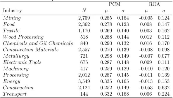
We use two measures of prot rate in the analyses: price-cost margin (PCM), which is dened as revenue minus costs relative to revenue, and return on assets (ROA), which is dened as operating prots divided by the assets of the rm. As can be seen from Table 2, rms from highly concentrated industries (e.g., Mining, Metallurgy, and Energy) tend to have a higher average level of PCM but much lower ROA. Interestingly, these same industries also have characteristics that impede entry or limit rivalry among members.

Furthermore, rms from these industries are commonly heavily subsidized in Ukraine.

Due to anticipated problems with misreporting of company prot, we prefer to use both measures of prot in the analysis. As rms are likely to report downward-biased values of their prot, ROA may be a more inaccurate measure of prot in an emerging economy compared to an advanced one. The price-cost margin is likely to be a more

7The CCEA (Classication of the Categories of Economic Activity).

8Van Phu et al. (2004) investigate the performance of German rms in the business-related service sector. They conclude that age and the degree of diversication have a negative impact on rm performance; additionally, credit relations with several banks allow rms with declining sales to improve their situation.

(8)

reliable measure for tracking the real performance trends. Hence, in our analysis we use price-cost margin as the key variable.

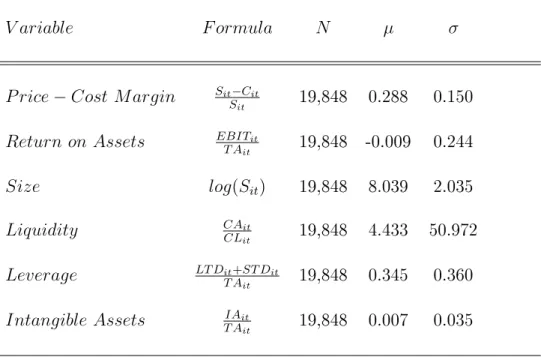
Table 3 contains some descriptive statistics. Price-cost margin has a mean of about 0.288 during the observed period. The negative value of average ROA (0.009) demonstrates the tendency of companies to report losses, although the large variation of this variable (0.244) shows a wide range of extremely polar values. The natural logarithm of sales is used as a proxy variable for rm size. We deliberately decided not to use number of employees as a measure of rm size as there is ample evidence about the frequently informal status of workers in transition economies.⁹ Leverage and liquidity are related to the debt literature of capital structure and reect the nancing opportunities of rms (Stephan et al. 2008). Mean leverage is about 34.5 percent of total liabilities. Liquidity is dened as the current assets to current liabilities ratio. This variable indicates that there is a considerable range of heterogeneity in regard to companies' cash constraints.

The IntangibleAssets variable is used to proxy goodwill, which is expected to have a great deal of inuence on rm performance. According to accounting standards, intangible assets include the value of patents, licenses, copyrights, and so forth. The mean of the intangible assets in total assets is only 0.007 for our sample, but the standard deviation (0.035) reveals notable variation of this variable across rms.

4 Empirical Results

4.1 Persistence of Prot

4.1.1 Markov Chain Approach

Prot persistence studies are typically based on estimation of rst-order or second-order autoregressive equations for rm protability. Tauchen (1986) suggests a discrete-value Markov chain analysis as an alternative procedure to approximate a continuous-valued autoregression. Quah (1993) applies the Markov chain method using transition probabil-

9See, for instance Kupets (2006).

(9)

ities matrices to investigate how income levels converge across dierent countries.¹⁰ We use the Markov chain approach in our analysis to explore the convergence and mobility of Ukrainian rm prot rates.

Lety_s^tdenote the prot rate of rm sat timet. A discrete-time Markov chain process requires that the following relation

P{y^t+1_s =j|y_s^t =i}=pij

hold for the sequence {y_s⁰, y_s¹...}, meaning that this is a stochastic process such that the probability p_ij of a random variable ybeing in the state j at any point of timet+ 1 depends only on the state i it has been in at point of time i. In other words, future developments during any transition periodt tot+ 1depend only on the value int. Thus, the transition among classes can be described as:

F_y^t+1 =P ·F_y^t, (1)

where Fy denotes the rm protability distribution at time t and t+ 1, respectively.

The discrete-time Markov chains allow tracing the development of rm behavior over time and examining intra-distribution mobility as well as persistence of rm protability.

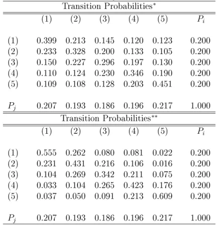
Under this approach, transition probability matrices can be estimated, which provide useful information regarding persistence as they describe the probability that a rm switches from one prot class to another. To obtain valid estimates and reasonable transition probabilities, two important prerequisites must be met: (i) time invariance of the data-generating process and (ii) a suciently large number of observations. The latter imposes additional requirement on the formation of optimal bandwidth. Taking into account the structure of our data, it is reasonable to dene ve, equally sized groups so as to meet the requirements of the Markov process: (1) the least protable rms; (2) low protable rms; (3) protable rms; (4) high protable rms; and (5) the most protable rms. Accordingly, the rst and second groups comprise companies with low

10A similar technique is developed in Quah (1996), Bickenbach and Bode (2003), Ces (2003) and Geppert and Stephan (2008).

(10)

prot rates, while the fourth and the fth classes are rms that have above-average prot.

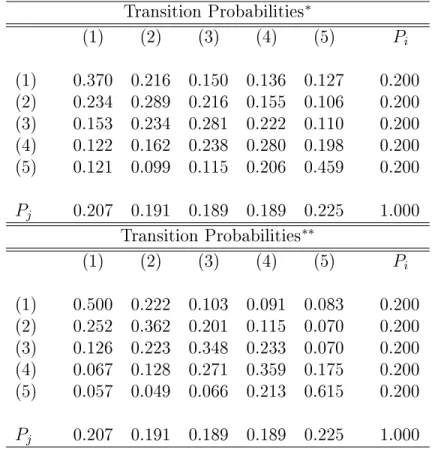
The transition probability matrices are estimated using the sample of rms for yearly transition periods (Tables 4 and 5 for PCM and ROA, respectively). In the case of strong prot persistency, all elements on the main diagonal should be close to 1. Thus, since the elements on the diagonal have values above 0.2, the results show a moderate persistence of prots. However, we nd a stronger persistence in the low and high prot classes, where the transition probability is around 0.4 (Bickenbach and Bode 2003).

The so-called half-life coecient is a useful tool for evaluating the mobility of rms across prot classes (Shorrocks 1978). The half-life coecients suggest the speed of convergence toward the equilibrium distribution for a Markov chain with transition matrix P.¹¹ In our case, the half-life coecients imply a relatively quick convergence:

the equilibrium state will be achieved after two years.

It is useful to compare these results with predicted outcomes/probabilities conditioned on the determinants of prot. To this end, multinomial logit regressions are employed despite the ordinal scale of our dependent variable.¹² The reason for employing this technique is to obtain the predicted transition probabilities of inter-group movements (Tables 4 and 5 for PCM and ROA, respectively). The results corroborate the prior conclusions as the elements of the new transition matrix gather along the main diagonal. However, conditioned outcomes show a considerably higher level of persistence and a longer time of convergence for both measures of protability (about ve years for PCM and about three and half years for ROA). Taken together, our ndings of a moderate level of persistence and a slow speed of adjustment to the steady-state value are in contrast to those of Glen and Singh (2003).

11Half-life measure: h=⁻_log|λ^log(2)

2|, whereλ₂ is the second largest eigenvalue of the transition matrix.

12The estimations of the multinomial regressions are available upon request.

(11)

4.1.2 Speed of Convergence: Robustness Check

The issue of prot persistence is usually analyzed as a time-series problem because in the structural model prot persistence is dominated by the impact of past prots (Goddard and Wilson (1999)). The majority of relevant studies implement the following empirical model:

π_it =α_i+λ_iπi,t−1+u_it (2)

where πit is normalized to the industry average prot of rm i in a given period t, α_i and λ_i denote the parameter of the lagged dependent variable, and u_it is i.i.d error term.

Empirical research is chiey interested in the estimation of λ_i, as it indicates the speed of adjustment. If λ_i is close to 1 it means that there is slow adjustment or, in other words, a high persistence of prot in successive periods. However, if λ_i has a value close to 0, it suggests that the prot level in the previous period does not aect the prot level in the current period, hence indicating the absence of prot persistence.

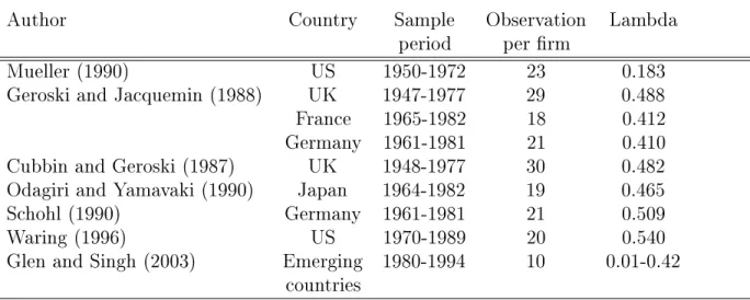
Goddard and Wilson (1999) summarize the most prominent studies in this eld (Table 1). Mueller (1990), for instance, using a sample of U.S. corporations, nds that the speed of adjustment is about 0.18 on average, which is a low value and thus can be viewed as a deviation from the more usual trend. However, he states that the long-run prot rates dier signicantly across rms and that the deviation of their prot above the norm appears to be quite stable for a remarkably high share of the rms (69 percent).

Comparing the outcomes across advanced countries, the main conclusion of Glen and Singh (2003) is that the persistency of prot rate for developing countries is lower than that of companies in advanced countries.

To provide additional evidence on the persistence of prot in emerging markets we use the GMM-SYS estimation technique as an alternative to the commonly applied regression methods in prot persistence studies. The model is specied as:

π_it =λπi,t−1+x⁰_itβ+u_it, i= 1, . . . , N, t= 1, . . . , T (3)

(12)

Table 1: Summary of prot persistence studies

Author Country Sample Observation Lambda

period per rm

Mueller (1990) US 1950-1972 23 0.183

Geroski and Jacquemin (1988) UK 1947-1977 29 0.488

France 1965-1982 18 0.412

Germany 1961-1981 21 0.410

Cubbin and Geroski (1987) UK 1948-1977 30 0.482

Odagiri and Yamavaki (1990) Japan 1964-1982 19 0.465

Schohl (1990) Germany 1961-1981 21 0.509

Waring (1996) US 1970-1989 20 0.540

Glen and Singh (2003) Emerging 1980-1994 10 0.01-0.42 countries

Source: Goddard and Wilson (1999), except Glen and Singh (2003)

where x_it is a vector of exogenous regressors, u_it =µ_i+ν_it,µ_i is a xed-eect, andν_it is a random disturbance.

We include the variables described in the previous section to control for important inuences on the prot rate. The size of company, intangible assets, and liquidity are presumably the most inuential determinants of protability of rms in emerging markets. Ownership structure and regional dummies are expected to provide some further evidence on the peculiarities of a transition economy. Moreover, each equation includes the diversication, year, and industry dummy variables.

The econometric model is estimated using the two-step GMMSYSTEM dynamic panel estimator, which is the preferred estimator in our case, as it, unlike the usual GMM estimator, uses not only transformed equations but also combines transformed equations with level equations (see Blundell and Bond (1998)). The models are estimated using the orthogonal transformation to remove individual rm eects. To check the validity of the instruments, we perform Hansen's test of overidentifying restrictions, which is asymptotically distributed as χ²(k) wherek denotes the number of overidentifying restrictions. Note that the GMM estimates are valid only if νit errors are serially

(13)

uncorrelated. Therefore, we present the test statistics for rst-order and second-order serial correlation.¹³

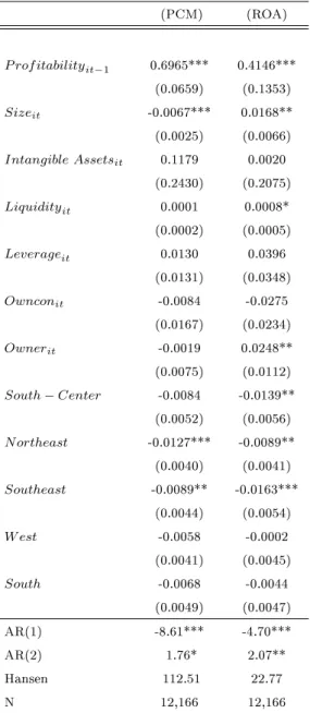
Table 6 reports the estimated parameters of the determinants of protability measured by PCM and ROA. All estimated coecients are in line with our predictions.

The main focus of our investigation is on the speed of prot adjustment which can be calculated from the estimated parameters on lagged prot rates. The estimated λi is 0.4146 and 0.6965 for ROA and PCM respectively (Table 6). These parameters enable the calculation of the half-life measure, which can be used as a further robustness check.

We achieve results very similar to those obtained from the previous Markov chain technique. The implied time of convergence for PCM is a little bit longer (about six years) compared to the Markov chain result, while the adjustment time for ROA varies between the results for unconditional and conditional transition matrices of the Markov chain approach. Thus, the results of the dynamic panel data analysis regarding the persistence and speed of adjustment of prot do not agree with the results for emerging markets reported in Glen and Singh (2003).

The estimation results furthermore suggest that regional eects are important for explaining dierences in prot rates (Table 6). Compared to rms located in the reference region (North-Center), rms located in the other Ukrainian regions have a signicantly lower level of protability. This nding is in accord with the results of Schnytzer and Andreyeva (2002), who report a permanent better performance of companies located in central regions of Ukraine. The estimation results for ownership structure support the view that individual ownership is positively associated with performance in Ukraine (Pivovarsky 2001). However, this appears to be true only for ROA, not for protability in terms of PCM.

13We apply the Windmeijer (2005) nite sample correction using the XTABOND2 module of the STATA package. In case of GMM-SYS the matrix of instruments for all rms estimation includes (P rof itability)_t−2to(P rof itability)_t−4,(Size)_t−1to(Size)_t−3,(Intangible Assets)_t−1to(Intangible Assets)_t−3, and(Liquidity)_t−1to(Liquidity)_t−3, and∆(P rof itability)_t−4,∆(Size)_t−3,∆(Intangible Assets)_t−3, and∆(Liquidity)_t−3. See help for XTABOND2 Roodman (2006) for matrix of instruments selection.

(14)

4.2 Determinants of Firm Prots

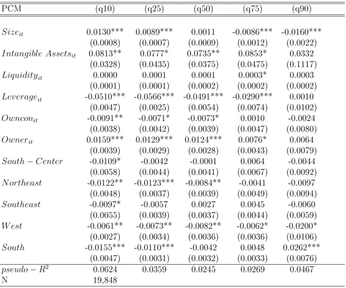
To study the determinants of prot in more detail, we perform quantile regression analyses (Koenker and Hallock 2001). For our purposes, estimation of linear models by quantile regressions is preferable over the usual regression methods for a number of reasons. First, quantile regression results are characteristically robust to outliers and heavy-tailed distributions (Buchinsky 1998). Second, the quantile regressions technique avoids the restrictive assumption that the error terms are identically distributed at all points of the conditional distribution. Avoiding this assumption allows us to capture rm heterogeneity in that the slope parameters can vary at dierent quantiles of the distribution of the dependent variable. An additional reason for using quantile regression methodology is if variables are skewed or not normally distributed. Note that the coecients from quantile regression can be interpreted as a marginal change in regressand at the certain quantile due to marginal change in particular regressor (Yasar et al. 2006).

Tables 7 and 10 report the results from the quantile regressions for PCM and ROA, respectively. From these tables, we can observe, rst, that the explanatory power of the models is higher for both the least and the most protable rms. As expected, the outcomes for ROA demonstrate a positive signicant association between protability and size, which is consistent with theory and also a plausible nding for transition countries in particular. Tybout (2000), for example, points out that due to particular features of emerging markets, large rms have some advantages: (i) policies favor larger companies, while inhibiting growth among small rms, (ii) as a rule, large-scale producers are selected for special subsidies, (iii) banks view larger companies as relatively less risky and cheaper to service, and thus these companies are given preferential access to credit, (iv) protectionist trade policies are more likely to favor large rms, (v) and capital- intensive rms can lobby the government more vigorously.

A signicant positive eect of rm size on PCM is found only for lower quantiles.

The protability of rms with average levels of PCM is not sensitive to rm size, while negative coecients for size are obtained for their more protable counterparts. This implies that the size of less protable rms is of great importance for enhancing PCM.

(15)

However, more protable rms try to reduce size so as to maintain a higher PCM. Ap- parently, this issue is related to the eective scale question, since the most protable companies do not benet from large size in achieving extra PCM and they are inclined to report higher levels of ROA. This issue is especially notable as large relatively unprof- itable rms have a much better chance of surviving compared to protable but smaller companies (Singh 2003).

Glen and Singh (2004) argue that emerging market companies have a higher level of xed assets than their counterparts in advanced markets. This is an important state- ment, since high prot can be maintained only by sustained innovation (Mueller 1990).

However, Galbreath and Galvin (2008) emphasize that tangible assets cannot be the source of permanent competitive advantage because they are observable factors and, thus, can be easily imitated by rivals, and that it is only reputation, patents, and other intangible assets that result in abnormal prot. Therefore, it is interesting to look at whether the share of intangible assets in the structure of total (or xed assets) allows rms to obtain higher prot. Our results demonstrate that PCM is positively related to intangible assets, while there is no eect of this variable on ROA.

An interesting aspect of the prot persistence issue is companies' capability to smooth cash-ow shocks. To estimate this eect, we dene the liquidity ratio, which character- izes rms' cash constraints.¹⁴ Garner et al. (2002) note that volatility of cash ows inuences the market value of rms. However, a positive and signicant inuence is obtained only at the 75 percent quantile for PCM.

Several studies stress the crucial impact of agency costs and related problems with corporate governance that ensue from unresolved ownership relations in Ukraine. For instance, Estrin and Rosevear (1999) argue that outsiders have no inuence on rm performance in Ukraine due to the underdeveloped capital markets and the dispersed ownership structure. Schnytzer and Andreyeva (2002) nd that ownership concentration improves the performance of Ukrainian companies. In contrast to these studies, our estimation provides evidence of a signicant and robust negative impact of concentrated

14Konings et al. (2003) nd a stronger persistence of soft budget constraints for rms in less developed countries.

(16)

ownership on protability ratios despite poor protection of minority ownership rights and weak capital markets. However, this can be explained by cross-shareholding that leads to reallocation of rm resources to optimize joint benets of companies within the business group. Khanna and Palepu (2000) point out that aliated companies can face a situation of misallocation of capital when the cash ow generated by protable rms within the group is invested in unprotable ventures, even though this may not be in interest of minor shareholders. Moreover, Baum et al. (2008) demonstrate that Ukrainian banks with political aliations operate with an objective function dierent from that of strict prot maximization. The inuence of ownership structure on prot persistence is additionally examined by controlling for the type of main stakeholder.¹⁵ As predicted, if the dominant shareholder is a private individual, there is better rm performance. The behavior of the most (least) protable companies is totally dierent from the main group of rms in the case of PCM (ROA) as it is not sensitive to the impact of ownership structure.

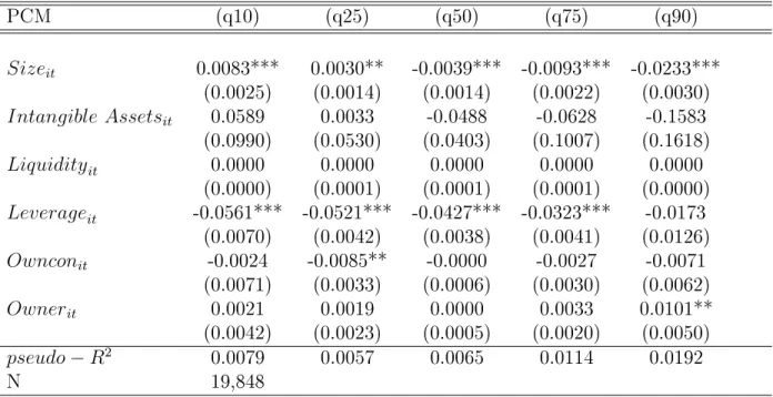
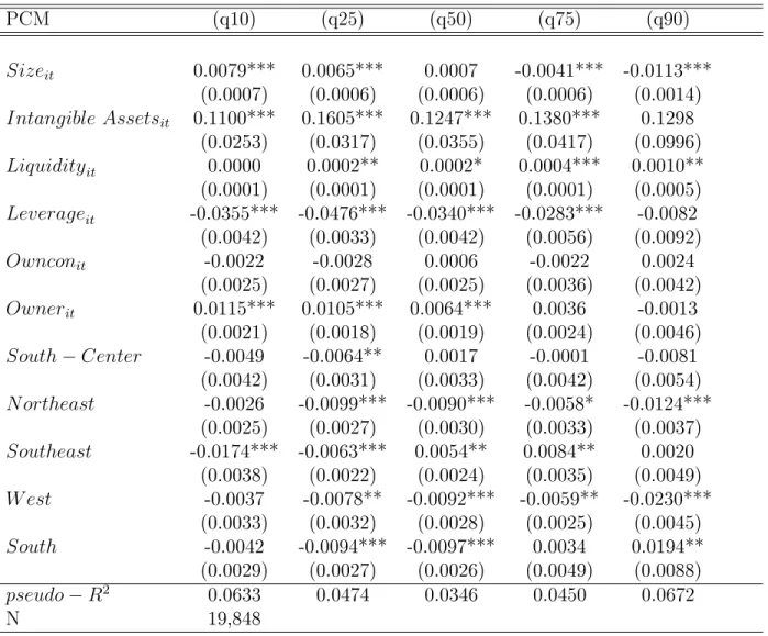
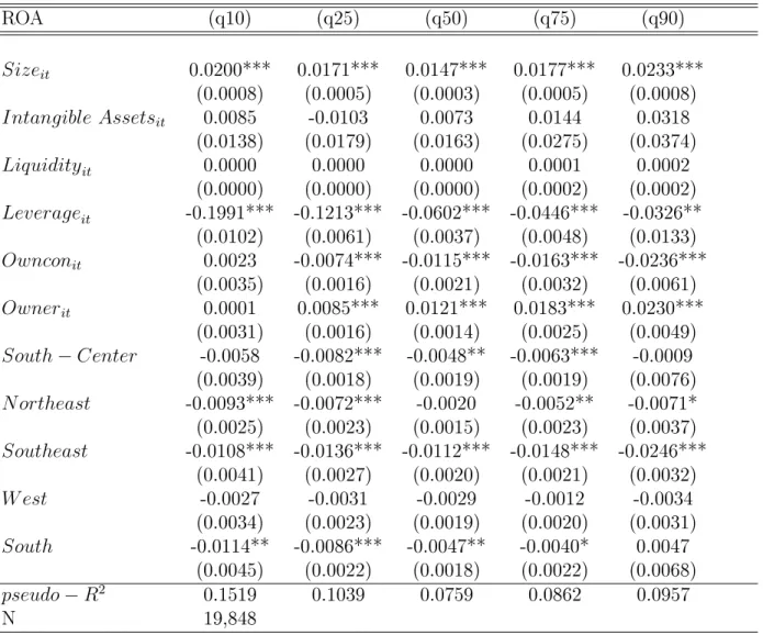
To gain a deeper insight into the processes aecting the prot rates, we run quantile regressions for rm-specic averages (between-rm regressions)and for within-rm transformed variables (within-rm regressions). The results for within-rm quantile regressions are reported in8 and 11 for PCM and ROA, respectively. Tables 9 and 12 set out the outcomes for the between-rm quantile calculations, the most interesting of which is the positive signicant coecients for liquidity, a nding that conrms our previous hypothesis. The signicant inverse relation between ROA and intangible assets for regressions based on within transformed variables is found for the rms with the lowest and the highest rates of prots. This result implies regardless of the fact that these rms have invested heavily in patents and licenses, they still perform poorly. Very similar results were found by Coad and Rao (2008). Finally, it should be mentioned that models based on rm-specic averages have more explanatory power and validate the principal tendencies described above for both measures of prot rate.

15In general, corporate owners are assumed to have lower cost of monitoring the rm's management because of greater expertise. Garner et al. (2002) note that the market value of a company is sensitive to the percentage of institutional ownership.

(17)

5 Conclusions

The aim of our paper is to provide evidence on the hypothesis put forward by Glen and Singh (2003) that the persistence of prot is lower in emerging markets compared to advanced ones. We use a panel data set on balance sheets and income statements of open joint stock Ukrainian companies during 19992006 in our analysis. The outcomes of the Markov chain analysis show evidence of a moderate or high level of prot persistence in Ukraine. This nding holds for both measures of protabilityprice-cost margin and return on assets. Thus, our results cast doubt on Glen and Singh's (2003) hypothesis that competition is more intense in emerging markets compared to advanced economies.

To complement and further substantiate these ndings, we use dynamic panel data techniques, enabling us to evaluate the speed of prot convergence in Ukraine. The estimates vary between 0.415 and 0.697 for return on assets and price-cost margin, respectively, implying a comparatively low speed (six years) of adjustment of prots to their steady-state value. Overall, the ndings for Ukranian rms do not signicantly dier from results that have been found in other empirical studies for rms in more advanced economies, which is a surprising outcome of our study.

Regarding the determinants of prot, one noteworthy result is the signicant impact of ownership structure and regional location of rms. Firms located in the North-Center of Ukraine have, c.p., a higher protability than rms located in other regions. An unexpected negative relationship between prot and ownership concentration appears to be related to the misallocation of nancial resources within business groups (Khanna and Palepu 2000) and to the eect of dierent objective functions for prot maximization of Ukrainian rms (Baum et al. 2008). However, the ownership concentration exerts a direct inuence on prot if the blocking share belongs to a private individual, a nding that is in agreement with Estrin and Wright (1999).

Taking into account rm heterogeneity, it is worth noting the varying impact of prot determinants at the high and low ends of the prot distribution. The results of the quantile regressions indicate that cross-shareholding and agency issues play a role for explaining prot in emerging markets.

(18)

References

Baum, C. F., Caglayan, M., Schäfer, D., Talavera, O. (2008): Political patronage in Ukrainian banking, Economics of Transition 16 (3), 537557.

Bickenbach, F., Bode, E. (2003): Evaluating the Markov property in studies of economic convergence, International Regional Science Review 26, 363392.

Blundell, R., Bond, S. (1998): Initial conditions and moment restrictions in dynamic panel data models, Journal of Econometrics 87 (1), 115143.

Buchinsky, M. (1998): Recent advances in quantile regression models: a practical guide for empirical research, Journal of Human Resources 30 (1), 88126.

Caves, R., Porter, M. (1977): From entry barriers to mobility barriers, Quarterly Journal of Economics 91, 241262.

Ces, E. (1998): Persistence in protability and in innovative activities, Working paper, Bocconi University and University of Bergamo.

Ces, E. (2003): Is there persistence in innovative activities?, International Journal of Industrial Organization 21, 489515.

Coad, A., Rao, R. (2008): The convergence of prots in the long-run: Inter-rm and inter-industry comparisons, Research Policy 37 (4), 633648.

Cubbin, J., Geroski, P. (1987): The convergence of prots in the long-run: Inter-rm and inter-industry comparisons, The Journal of Industrial Economics 35 (4), 427442.

Estrin, S., Rosevear, A. (1999): Enterprise performance and corporate governance in Ukraine, Journal of Comparative Economics 27, 442458.

Estrin, S., Wright, M. (1999): Corporate governance in the former Soviet Union: An overview, Journal of Comparative Economics 27, 398421.

(19)

Galbreath, J., Galvin, P. (2008): Firm factors, industry structure and performance variation: New empirical evidence to a classic debate, Journal of Business Research 61, 109117.

Garner, J. L., Nam, J., Ottoo, R. E. (2002): Determinants of corporate growth opportunities of emerging rms, Journal of Economics and Business 54, 7393.

Geppert, K., Stephan, A. (2008): Regional disparities in the European union: Conver- gence and aglomeration, Papers in Regional Science 87, 193217.

Geroski, P. A., Jacquemin, A. (1988): The persistence of prots: A European compar- ison, The Economic Journal 98, 375389.

Glen, J., Singh, A. (2003): Corporate protability and the dynamics of competition in emerging markets: A time series analysis, The Economic Journal 113, 465484.

Glen, J., Singh, A. (2004): Comparing capital structures and rates of return in developed and emerging markets, Emerging Markets Review 5 (2), 161192.

Goddard, J. A., Wilson, J. O. S. (1999): The persistence of prot: a new empirical interpretation, International Journal of Industrial Organization 17 (5), 663687.

Khanna, T., Palepu, K. (2000): Is group aliation protable in emerging markets? An analysis of diversied Indian business groups, Journal of Finance LV (2), 867891.

Koenker, R., Hallock, K. F. (2001): Quantile regression, Journal of Economic Perspec- tives 15 (4), 143156.

Konings, J., Rizov, M., Vandenbussche, H. (2003): Investment and nancial constraints in transition economies: micro evidence from Poland, the Czech Republic, Bulgaria and Romania, Economics Letters 78, 253258.

Kupets, O. (2006): Determinants of unemployment duration in Ukraine, Journal of Comparative Economics 34, 228247.

(20)

McGahan, A. M. (1999): The performance of US corporations: 1981-1994, The Journal of Industrial Economics 47 (4), 373398.

McGahan, A. M., Porter, M. E. (1999): The persistence of shocks to protability, The Review of Economics and Statistics 81 (1), 143153.

Mueller, D. C. (1977): The persistence of prots above the norm, Economica 44, 369380.

Mueller, D. C. (1986): Prots in the Long-run, Cambridge University Press.

Mueller, D. C. (1990): The Dynamics of Company Prots: An International Compari- son, Cambridge University Press.

Pivovarsky, A. (2001): How does privatization work? Ownership concentration and enterprise performance in Ukraine, Working paper 42, IMF.

Quah, D. (1993): Empirical cross-section dynamics in economic growth, European Economic Review 37, 426434.

Quah, D. (1996): Empirics for economic growth and convergence, European Economic Review 40, 13531375.

Roodman, D. (2006): Xtabond2: Stata module to extend xtabond dynamic panel data estimator, Statistical Software Components, Boston College Department of Eco- nomics.

Schnytzer, A., Andreyeva, T. (2002): Company performance in Ukraine: is this a market economy? Economic Systems 26, 8398.

Shorrocks, A. (1978): The measurement of mobility, Econometrica 46 (5), 10131024.

Singh, A. (2003): Competition, corporate governance and selection in emerging markets, The Economic Journal 113, 443464.

(21)

Stephan, A., Talavera, O., Tsapin, A. (2008): Corporate debt maturity choice in transition nancial markets, CESIS Working Paper 125, Royal Institute of Technology.

Tauchen, G. (1986): Finite state markov-chain approximizations to univariate and vector autoregressions, Economics Letters 20, 177181.

Tybout, J. R. (2000): Manufacturing rms in developing countries: How well do they do, and why? Journal of Economic Literature 38, 1144.

Van Phu, N., Kaiser, U., Laisney, F. (2004, The performance of German rms in the business-related service sectors: a dynamic analysis, Journal of Business and Economic Statistics 22, 274295.

Waring, G. F. (1996): Industry dierences in the persistence of rm-specic returns, The American Economic Review 86 (5), 12531265.

Windmeijer, F. (2005): A nite sample correction for the variance of linear ecient two-step GMM estimators, Journal of Econometrics 126, 2551.

Yasar, M., Nelson, C. H., Rejesus, R. (2006): Productivity and exporting status of manufacturing rms: Evidence from quantile regressions, Review of World Economics 142, 675694.

Yurtoglu, B. Burcin (2004): Persistence of rm-level protability in Turkey, Applied Economics 36, 615625.

(22)

Table 2: Descriptive Statistics: Prot Rates across Industries

PCM ROA

Industry N µ σ µ σ

M ining 2,759 0.285 0.164 -0.005 0.124

F ood 2,362 0.278 0.123 0.008 0.147

T extile 1,170 0.269 0.140 0.003 0.162

W ood P rocessing 518 0.288 0.144 0.012 0.112 Chemicals and Oil Chemicals 840 0.290 0.132 0.016 0.170 Consturction M aterials 2,557 0.270 0.139 -0.008 0.098

M etallurgy 721 0.298 0.149 -0.007 0.077

Electronic T ools 675 0.287 0.148 0.009 0.111

M achinery 417 0.259 0.129 -0.010 0.120

P rocessing 2,012 0.287 0.145 -0.011 0.139

Energy 3,549 0.335 0.165 -0.013 0.153

Construction 2,124 0.252 0.149 -0.053 0.632

T ransport 144 0.332 0.168 0.006 0.224

Note: Price-cost margin variable (PCM) is dened as sales minus cost divided by sales. Return on Assets (ROA) is constructed as EBIT to assets ratio.

(23)

Table 3: Descriptive Statistics

V ariable F ormula N µ σ

P rice−Cost M argin ^S^it_S^−C^it

it 19,848 0.288 0.150 Return on Assets ^EBIT_{T A} ^it

it 19,848 -0.009 0.244

Size log(S_it) 19,848 8.039 2.035

Liquidity ^CA_CL^it

it 19,848 4.433 50.972 Leverage ^{LT D}^it_{T A}^{+ST D}^it

it 19,848 0.345 0.360 Intangible Assets _{T A}^IA^it

it 19,848 0.007 0.035

Note: Price-cost margin variable (PCM) is dened as sales minus cost divided by sales. Return on Assets (ROA) is constructed as EBIT to assets ratio. Size is measured by logarithm of sales. Liquidity is dened as the current assets to current liabilities ratio. Leverageis the rm's debt to total assets ratio. Intangible Assets is calculated as a share of intangible assets in total assets.

(24)

Table 4: Transition Probability Matrices: Result for PCM Transition Probabilities^∗

(1) (2) (3) (4) (5) Pi

(1) 0.399 0.213 0.145 0.120 0.123 0.200 (2) 0.233 0.328 0.200 0.133 0.105 0.200 (3) 0.150 0.227 0.296 0.197 0.130 0.200 (4) 0.110 0.124 0.230 0.346 0.190 0.200 (5) 0.109 0.108 0.128 0.203 0.451 0.200 P_j 0.207 0.193 0.186 0.196 0.217 1.000

Transition Probabilities^∗∗

(1) (2) (3) (4) (5) P_i

(1) 0.555 0.262 0.080 0.081 0.022 0.200 (2) 0.231 0.431 0.216 0.106 0.016 0.200 (3) 0.104 0.269 0.342 0.211 0.075 0.200 (4) 0.033 0.104 0.265 0.423 0.176 0.200 (5) 0.037 0.050 0.091 0.213 0.609 0.200 P_j 0.207 0.193 0.186 0.196 0.217 1.000

Note:

Pi - initial probabilities.

Pj - destination probabilities.

∗ - unconditional probability.

∗∗ - conditional probability.

(1) the least protable rms; (2) low protable rms; (3) protable rms; (4) highly protable rms;

(5) the most protable rms.

(25)

Table 5: Transition Probability Matrices: Result for ROA Transition Probabilities^∗

(1) (2) (3) (4) (5) Pi

(1) 0.370 0.216 0.150 0.136 0.127 0.200 (2) 0.234 0.289 0.216 0.155 0.106 0.200 (3) 0.153 0.234 0.281 0.222 0.110 0.200 (4) 0.122 0.162 0.238 0.280 0.198 0.200 (5) 0.121 0.099 0.115 0.206 0.459 0.200 P_j 0.207 0.191 0.189 0.189 0.225 1.000

Transition Probabilities^∗∗

(1) (2) (3) (4) (5) P_i

(1) 0.500 0.222 0.103 0.091 0.083 0.200 (2) 0.252 0.362 0.201 0.115 0.070 0.200 (3) 0.126 0.223 0.348 0.233 0.070 0.200 (4) 0.067 0.128 0.271 0.359 0.175 0.200 (5) 0.057 0.049 0.066 0.213 0.615 0.200 P_j 0.207 0.191 0.189 0.189 0.225 1.000

Note:

Pi - initial probabilities.

Pj - destination probabilities.

∗ - unconditional probability.

∗∗ - conditional probability.

(1) the least protable rms; (2) low protable rms; (3) protable rms; (4) highly protable rms;

(5) the most protable rms.

(26)

Table 6: Determinants of Prot

Dependent Variable: P rof it rateit

(PCM) (ROA)

P rof itability_it−1 0.6965*** 0.4146***

(0.0659) (0.1353)

Sizeit -0.0067*** 0.0168**

(0.0025) (0.0066) Intangible Assetsit 0.1179 0.0020

(0.2430) (0.2075)

Liquidity_it 0.0001 0.0008*

(0.0002) (0.0005)

Leverage_it 0.0130 0.0396

(0.0131) (0.0348)

Ownconit -0.0084 -0.0275

(0.0167) (0.0234)

Ownerit -0.0019 0.0248**

(0.0075) (0.0112) South−Center -0.0084 -0.0139**

(0.0052) (0.0056)

N ortheast -0.0127*** -0.0089**

(0.0040) (0.0041)

Southeast -0.0089** -0.0163***

(0.0044) (0.0054)

W est -0.0058 -0.0002

(0.0041) (0.0045)

South -0.0068 -0.0044

(0.0049) (0.0047)

AR(1) -8.61*** -4.70***

AR(2) 1.76* 2.07**

Hansen 112.51 22.77

N 12,166 12,166

Note: Price-cost margin variable (PCM) is dened as sales minus cost divided by sales. Return on Assets (ROA) is constructed as EBIT to total assets ratio. Size is measured by logarithm of sales.

Intangible Assets is calculated as a share of intangible assets in total assets. Liquidityis dened as the current assets to current liabilities ratio. Leverageis the rm's debt to total assets ratio. Ownconis a dummy variable that takes value of one if the rm has concentrated ownership structure. Owner is a dummy variable which equals one if dominant shareholder is an individual.

Each equation includes year, industry, and diversication dummy variables. Reference category for regional eects is North-Center. Asymptotic robust standard errors are reported in the brackets. Es-24

(27)

Table 7: Determinants of Corporate Prot Dependent Variable: P CM_it

PCM (q10) (q25) (q50) (q75) (q90)

Size_it 0.0130*** 0.0089*** 0.0011 -0.0086*** -0.0160***

(0.0008) (0.0007) (0.0009) (0.0012) (0.0022) Intangible Assets_it 0.0813** 0.0777* 0.0735** 0.0853* 0.0332

(0.0328) (0.0435) (0.0375) (0.0475) (0.1117) Liquidity_it 0.0000 0.0001 0.0001 0.0003* 0.0003

(0.0001) (0.0001) (0.0002) (0.0002) (0.0002) Leverage_it -0.0510*** -0.0566*** -0.0491*** -0.0290*** 0.0010

(0.0047) (0.0025) (0.0054) (0.0074) (0.0102) Owncon_it -0.0091** -0.0071* -0.0073* 0.0010 -0.0024

(0.0038) (0.0042) (0.0039) (0.0047) (0.0080) Owner_it 0.0159*** 0.0129*** 0.0124*** 0.0076* 0.0064

(0.0039) (0.0029) (0.0028) (0.0043) (0.0079) South−Center -0.0109* -0.0042 -0.0001 0.0064 -0.0044

(0.0058) (0.0044) (0.0041) (0.0067) (0.0092) N ortheast -0.0122** -0.0123*** -0.0084** -0.0041 -0.0097

(0.0048) (0.0037) (0.0039) (0.0049) (0.0094) Southeast -0.0097* -0.0057 0.0027 0.0045 -0.0060

(0.0055) (0.0039) (0.0037) (0.0044) (0.0059) W est -0.0061** -0.0073** -0.0082** -0.0062* -0.0200*

(0.0027) (0.0034) (0.0036) (0.0036) (0.0106) South -0.0155*** -0.0110*** -0.0042 0.0048 0.0262***

(0.0047) (0.0031) (0.0032) (0.0033) (0.0076) pseudo−R² 0.0624 0.0359 0.0245 0.0269 0.0467

N 19,848

Note: Price-cost margin variable (PCM) is dened as sales minus cost divided by sales. Size is measured by logarithm of sales. Intangible Assets is calculated as a share of intangible assets in total assets.

Liquidityis dened as the current assets to current liabilities ratio. Leverageis the rm's debt to total assets ratio. Ownconis a dummy variable that takes value of one if the rm has concentrated ownership structure. Owneris a dummy variable which equals one if dominant shareholder is an individual.

Each equation includes year, industry, and diversication dummy variables. Reference category for regional eects is North-Center. Standard errors are reported in the parentheses.

* signicant at 10%; ** signicant at 5%; *** signicant at 1%.

(28)

Table 8: Determinants of Corporate Prot: Result for Within Transformed Variables Dependent Variable: P CMit

PCM (q10) (q25) (q50) (q75) (q90)

Size_it 0.0083*** 0.0030** -0.0039*** -0.0093*** -0.0233***

(0.0025) (0.0014) (0.0014) (0.0022) (0.0030) Intangible Assets_it 0.0589 0.0033 -0.0488 -0.0628 -0.1583

(0.0990) (0.0530) (0.0403) (0.1007) (0.1618) Liquidity_it 0.0000 0.0000 0.0000 0.0000 0.0000

(0.0000) (0.0001) (0.0001) (0.0001) (0.0000) Leverage_it -0.0561*** -0.0521*** -0.0427*** -0.0323*** -0.0173

(0.0070) (0.0042) (0.0038) (0.0041) (0.0126) Owncon_it -0.0024 -0.0085** -0.0000 -0.0027 -0.0071

(0.0071) (0.0033) (0.0006) (0.0030) (0.0062)

Owner_it 0.0021 0.0019 0.0000 0.0033 0.0101**

(0.0042) (0.0023) (0.0005) (0.0020) (0.0050) pseudo−R² 0.0079 0.0057 0.0065 0.0114 0.0192

N 19,848

Each equation includes year, industry, and diversication dummy variables. Standard errors are reported in the parentheses.

(29)

Table 9: Determinants of Corporate Prot: Result for Between Transformed Variables Dependent Variable: P CM_it

PCM (q10) (q25) (q50) (q75) (q90)

Size_it 0.0079*** 0.0065*** 0.0007 -0.0041*** -0.0113***

(0.0007) (0.0006) (0.0006) (0.0006) (0.0014) Intangible Assets_it 0.1100*** 0.1605*** 0.1247*** 0.1380*** 0.1298

(0.0253) (0.0317) (0.0355) (0.0417) (0.0996) Liquidity_it 0.0000 0.0002** 0.0002* 0.0004*** 0.0010**

(0.0001) (0.0001) (0.0001) (0.0001) (0.0005) Leverage_it -0.0355*** -0.0476*** -0.0340*** -0.0283*** -0.0082

(0.0042) (0.0033) (0.0042) (0.0056) (0.0092) Owncon_it -0.0022 -0.0028 0.0006 -0.0022 0.0024

(0.0025) (0.0027) (0.0025) (0.0036) (0.0042) Owner_it 0.0115*** 0.0105*** 0.0064*** 0.0036 -0.0013

(0.0021) (0.0018) (0.0019) (0.0024) (0.0046) South−Center -0.0049 -0.0064** 0.0017 -0.0001 -0.0081

(0.0042) (0.0031) (0.0033) (0.0042) (0.0054) N ortheast -0.0026 -0.0099*** -0.0090*** -0.0058* -0.0124***

(0.0025) (0.0027) (0.0030) (0.0033) (0.0037) Southeast -0.0174*** -0.0063*** 0.0054** 0.0084** 0.0020

(0.0038) (0.0022) (0.0024) (0.0035) (0.0049) W est -0.0037 -0.0078** -0.0092*** -0.0059** -0.0230***

(0.0033) (0.0032) (0.0028) (0.0025) (0.0045) South -0.0042 -0.0094*** -0.0097*** 0.0034 0.0194**

(0.0029) (0.0027) (0.0026) (0.0049) (0.0088) pseudo−R² 0.0633 0.0474 0.0346 0.0450 0.0672

N 19,848

(30)

Table 10: Determinants of Corporate Prot Dependent Variable: ROA_it

ROA (q10) (q25) (q50) (q75) (q90)

Size_it 0.0200*** 0.0171*** 0.0147*** 0.0177*** 0.0233***

(0.0008) (0.0005) (0.0003) (0.0005) (0.0008) Intangible Assets_it 0.0085 -0.0103 0.0073 0.0144 0.0318

(0.0138) (0.0179) (0.0163) (0.0275) (0.0374) Liquidity_it 0.0000 0.0000 0.0000 0.0001 0.0002

(0.0000) (0.0000) (0.0000) (0.0002) (0.0002) Leverage_it -0.1991*** -0.1213*** -0.0602*** -0.0446*** -0.0326**

(0.0102) (0.0061) (0.0037) (0.0048) (0.0133) Owncon_it 0.0023 -0.0074*** -0.0115*** -0.0163*** -0.0236***

(0.0035) (0.0016) (0.0021) (0.0032) (0.0061) Owner_it 0.0001 0.0085*** 0.0121*** 0.0183*** 0.0230***

(0.0031) (0.0016) (0.0014) (0.0025) (0.0049) South−Center -0.0058 -0.0082*** -0.0048** -0.0063*** -0.0009

(0.0039) (0.0018) (0.0019) (0.0019) (0.0076) N ortheast -0.0093*** -0.0072*** -0.0020 -0.0052** -0.0071*

(0.0025) (0.0023) (0.0015) (0.0023) (0.0037) Southeast -0.0108*** -0.0136*** -0.0112*** -0.0148*** -0.0246***

(0.0041) (0.0027) (0.0020) (0.0021) (0.0032)

W est -0.0027 -0.0031 -0.0029 -0.0012 -0.0034

(0.0034) (0.0023) (0.0019) (0.0020) (0.0031) South -0.0114** -0.0086*** -0.0047** -0.0040* 0.0047

(0.0045) (0.0022) (0.0018) (0.0022) (0.0068) pseudo−R² 0.1519 0.1039 0.0759 0.0862 0.0957

N 19,848

Note: Return on Assets (ROA) is constructed as EBIT to assets ratio. Size is measured by logarithm of sales. Intangible Assets is calculated as a share of intangible assets in total assets. Liquidity is dened as the current assets to current liabilities ratio. Leverageis the rm's debt to total assets ratio.

Ownconis a dummy variable that takes value of one if the rm has concentrated ownership structure.

Owneris a dummy variable which equals one if dominant shareholder is an individual.

(31)

Table 11: Determinants of Corporate Prot: Result for Within Transformed Variables Dependent Variable: ROAit

ROA (q10) (q25) (q50) (q75) (q90)

Size_it 0.0327*** 0.0281*** 0.0226*** 0.0251*** 0.0270***

(0.0018) (0.0012) (0.0010) (0.0013) (0.0022) Intangible Assets_it -0.1811** -0.0435 -0.0077 -0.0122 -0.1343*

(0.0808) (0.0365) (0.0232) (0.0280) (0.0728) Liquidity_it 0.0000** 0.0000 0.0000 0.0000 0.0000

(0.0000) (0.0000) (0.0000) (0.0000) (0.0000) Leverage_it -0.1920*** -0.1463*** -0.1233*** -0.1357*** -0.1690***

(0.0185) (0.0125) (0.0079) (0.0101) (0.0142) Owncon_it -0.0000 -0.0020 0.0020* 0.0027* -0.0001

(0.0044) (0.0017) (0.0010) (0.0014) (0.0046)

Owner_it -0.0030 -0.0014 0.0001 0.0016 0.0022

(0.0032) (0.0014) (0.0008) (0.0012) (0.0033) pseudo−R² 0.0680 0.0554 0.0465 0.0510 0.0527

N 19,848

Each equation includes year, industry, and diversication dummy variables. Standard errors are reported in the parentheses.

(32)

Table 12: Determinants of Corporate Prot: Result for Between Transformed Variables Dependent Variable: ROA_it

ROA (q10) (q25) (q50) (q75) (q90)

Size_it 0.0190*** 0.0158*** 0.0153*** 0.0185*** 0.0219***

(0.0005) (0.0003) (0.0005) (0.0003) (0.0004) Intangible Assets_it 0.0110 -0.0297*** -0.0098 -0.0284 0.1026***

(0.0156) (0.0101) (0.0157) (0.0285) (0.0272) Liquidity_it 0.0001 0.0001*** 0.0001 0.0002 0.0005**

(0.0000) (0.0000) (0.0001) (0.0002) (0.0002) Leverage_it -0.1344*** -0.0908*** -0.0632*** -0.0524*** -0.0368***

(0.0051) (0.0021) (0.0027) (0.0044) (0.0076) Owncon_it -0.0039 -0.0053*** -0.0088*** -0.0147*** -0.0247***

(0.0024) (0.0018) (0.0014) (0.0019) (0.0034) Owner_it 0.0090*** 0.0079*** 0.0105*** 0.0138*** 0.0179***

(0.0018) (0.0012) (0.0014) (0.0014) (0.0026) South−Center -0.0076*** -0.0080*** -0.0027 -0.0055*** -0.0043

(0.0027) (0.0023) (0.0018) (0.0021) (0.0036) N ortheast -0.0055* -0.0042*** -0.0055*** -0.0053*** -0.0152***

(0.0033) (0.0016) (0.0016) (0.0019) (0.0036) Southeast -0.0139*** -0.0111*** -0.0127*** -0.0169*** -0.0249***

(0.0020) (0.0010) (0.0015) (0.0015) (0.0036) W est -0.0052* -0.0035** 0.0007 0.0023 -0.0079***

(0.0027) (0.0017) (0.0015) (0.0021) (0.0029) South -0.0117*** -0.0113*** -0.0051*** -0.0021 -0.0064**

(0.0024) (0.0024) (0.0014) (0.0019) (0.0029) pseudo−R² 0.1714 0.1418 0.1183 0.1268 0.1423

N 19,848